Comparison Sorting Algorithms
Comparison Sorting Algorithms
Sorting is the task of rearranging a sequence so it obeys an order (usually ≤). Every comparison-based sort answers the same two questions differently: which pair do I compare next, and what do I do once I know the answer. The story of sorting is brute force → optimal: start with algorithms that re-examine information they already have (O(n²)), then derive algorithms that throw nothing away (O(n log n)).
Brute-force family — O(n²): bubble sort, selection sort, insertion sort. Each does roughly n² comparisons/swaps because each pass only learns one small fact (a max, or one correct position) and forgets everything else about the rest of the array.
Optimal family — O(n log n): merge sort and quicksort. Both exploit divide-and-conquer, but they divide differently — merge sort splits blindly and does the work on the merge; quicksort does the work on the split (partition) and then the recursion is free. That single design choice is the source of every trade-off between them, and we derive it below rather than asserting it.
1. Bubble Sort — repeatedly fix local violations
Idea: walk the array left to right; whenever adjacent elements are out of order, swap them. After one full pass, the largest element has 'bubbled' to the end. Repeat n times.
function bubbleSort(a):
  n = len(a)
  for i in 0..n-1:
    swapped = false
    for j in 0..n-2-i:
      if a[j] > a[j+1]:
        swap(a[j], a[j+1])
        swapped = true
    if not swapped: break   // already sorted, stop early
Complexity derivation: pass i does about (n−i) comparisons; summing i=0..n gives n + (n−1) + … + 1 = n(n+1)/2 = O(n²) comparisons and, worst case (reverse-sorted input), O(n²) swaps too. The early-exit flag makes best case O(n) when the input is already sorted — the only 'adaptive' feature bubble sort has.
When (not) to use it: bubble sort is not used in production anywhere — insertion sort dominates it on every axis (fewer writes, same worst case, simpler invariant). Its only remaining value is pedagogical: it is the simplest possible sort to trace by hand.
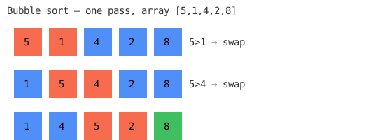
2. Selection Sort — find the minimum, place it once
Idea: for each position i, scan the unsorted remainder for its minimum and swap it into place. Unlike bubble sort, elements only move once they are known to be final.
function selectionSort(a):
  n = len(a)
  for i in 0..n-2:
    m = i
    for j in i+1..n-1:
      if a[j] < a[m]: m = j
    swap(a[i], a[m])
Complexity: comparisons are always (n−1)+(n−2)+…+1 = O(n²), regardless of input order — selection sort has no early-exit and no best case better than n²/2. But it makes at most n−1 swaps total, versus O(n²) for bubble sort.
When to use it: when writes are expensive relative to comparisons — e.g. sorting data on flash memory/EEPROM where each write wears the cell, or sorting an array of large structs by swapping pointers. If comparisons are cheap and writes are the bottleneck, selection sort's O(n) write bound beats every other O(n²) sort. Otherwise prefer insertion sort, which beats it on comparisons for partially-sorted input.
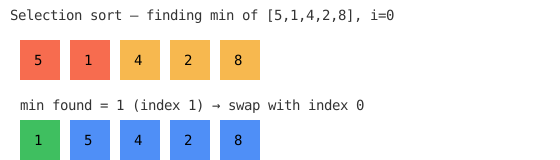
3. Insertion Sort — grow a sorted prefix
Idea: maintain a sorted prefix a[0..i-1]; take a[i] and slide it left past every element bigger than it.
function insertionSort(a):
  for i in 1..n-1:
    key = a[i]
    j = i - 1
    while j >= 0 and a[j] > key:
      a[j+1] = a[j]
      j -= 1
    a[j+1] = key
Complexity: worst case (reverse-sorted) is O(n²) — each key slides all the way to the front. Best case (already sorted) is O(n): the inner while loop never fires, so it's a single O(n) scan. This is the key property bubble and selection sort lack: insertion sort is adaptive — its running time scales with the number of inversions (out-of-order pairs), not blindly with n².
Why this matters beyond the algorithm itself: because insertion sort is fast on nearly-sorted data and has tiny constant factors (no recursion, no extra array, cache-friendly linear scans), production hybrid sorts fall back to it for small subarrays. Timsort (Python, Java's Collections.sort for objects) and Introsort (C++ std::sort, .NET) both switch from their O(n log n) algorithm to insertion sort once a partition shrinks below roughly 16–32 elements, because merge sort/quicksort's overhead (recursive calls, merge buffers, partition bookkeeping) costs more than n² comparisons do at that size.
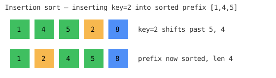
4. Merge Sort — split blindly, do the work on the merge
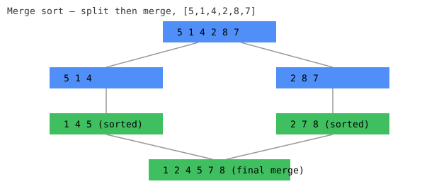
Idea: split the array in half regardless of content, recursively sort each half, then merge two sorted halves in one linear pass.
function mergeSort(a):
  if len(a) <= 1: return a
  mid = len(a) / 2
  left  = mergeSort(a[0:mid])
  right = mergeSort(a[mid:])
  return merge(left, right)

function merge(l, r):
  out = []
  i = j = 0
  while i < len(l) and j < len(r):
    if l[i] <= r[j]: out.append(l[i]); i += 1
    else:            out.append(r[j]); j += 1
  out.extend(l[i:]); out.extend(r[j:])
  return out
Complexity derivation: the recursion tree has log₂n levels (halving each time). Every level does a total of O(n) work across all merges at that level (each merge is linear in the combined size, and combined sizes across a level sum to n). Total = O(n) × O(log n) = O(n log n), guaranteed — this bound does not depend on input order, because the split point never depends on the data. The cost is the out buffer: merge needs O(n) auxiliary space per level (reusable across levels, so O(n) total), and merge sort is stable (equal keys keep their relative order) because the merge step always takes from the left run on ties.
5. Quicksort — do the work on the split, recursion is free
Idea: pick a pivot, partition the array so everything ≤ pivot ends up left of it and everything > pivot ends up right of it (pivot lands in its final position), then recurse on the two sides independently. Unlike merge sort there is no merge step — once partitioned, the two halves never need to be recombined.
Lomuto Partitioning Scheme
function quicksortLomuto(a, lo, hi):
  if lo >= hi: return
  p = partitionLomuto(a, lo, hi)
  quicksortLomuto(a, lo, p - 1)
  quicksortLomuto(a, p + 1, hi)

function partitionLomuto(a, lo, hi):
  pivot = a[hi]
  i = lo
  for j in lo..hi-1:
    if a[j] <= pivot:
      swap(a[i], a[j]); i += 1
  swap(a[i], a[hi])
  return i   // pivot's final index
Hoare Partitioning Scheme
Hoare partitioning uses two pointers starting at opposite ends of the array that walk toward each other, swapping elements that are on the wrong side of the pivot. Crucially: Hoare returns a split index p where all elements in a[lo..p] are ≤ pivot and all elements in a[p+1..hi] are ≥ pivot. Because the pivot element itself is not guaranteed to land at index p, the recursion partitions must be [lo..p] and [p+1..hi].
function quicksortHoare(a, lo, hi):
  if lo >= hi: return
  p = partitionHoare(a, lo, hi)
  quicksortHoare(a, lo, p)      // Recurse on left partition (including p)
  quicksortHoare(a, p + 1, hi)  // Recurse on right partition

function partitionHoare(a, lo, hi):
  pivot = a[lo]                 // Hoare traditionally uses first element (or random/median)
  i = lo - 1
  j = hi + 1
  while true:
    do: i += 1 while a[i] < pivot
    do: j -= 1 while a[j] > pivot
    if i >= j: return j
    swap(a[i], a[j])
Complexity derivation — why it's usually n log n but can be n²: partitioning a subarray of size k always costs O(k) (one linear scan). If every pivot splits its subarray roughly in half, the recursion tree has O(log n) levels, each doing O(n) total partition work → O(n log n), same shape as merge sort's derivation. But the split size depends entirely on the data: if the pivot is always the smallest or largest element (e.g. picking a[hi] as pivot on an already-sorted or reverse-sorted array), every partition produces a (1, k−1) split instead of (k/2, k/2). The recursion tree degenerates from log n levels to n levels, each doing O(k) work, giving 1+2+…+n = O(n²) — the same shape as bubble/selection sort's derivation. This worst case is not a corner case to shrug off: naive first-element or last-element pivot selection is adversarially triggerable by exactly the inputs engineers hit most (sorted or nearly-sorted data), which is why production quicksorts use randomized pivots or median-of-three, dropping the adversarial worst case to a vanishingly unlikely one while keeping the average case's small constant factors (in-place partitioning, no auxiliary buffer, better cache locality than merge sort).
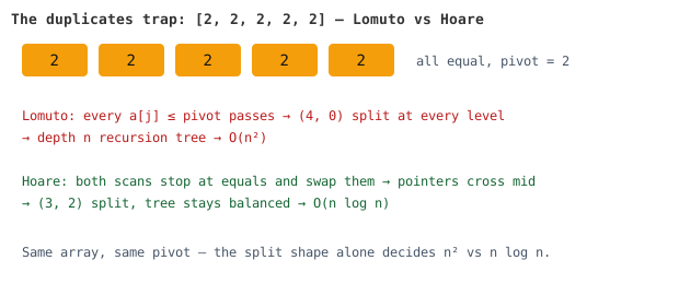
The Duplicate Elements Trap (Lomuto vs. Hoare): The Lomuto partition scheme shown above has another severe, silent failure mode: if the array consists entirely of duplicate or identical elements (e.g. [2, 2, 2, 2, 2]), Lomuto still performs a highly unbalanced split: every a[j] ≤ pivot test passes, so all elements land on one side and the recursion tree is (n−1, 0), level after level. Sorting an array of duplicates with Lomuto quicksort degrades to O(n²) time. The production-standard fix is Hoare Partitioning. Hoare uses two pointers starting at opposite ends that walk toward each other. Crucially, both scans (a[i] < pivot, a[j] > pivot) stop at elements equal to the pivot — and then swap them. Those seemingly wasted swaps of equal elements are exactly what spreads duplicates across both sides: on [2, 2, 2, 2, 2] the pointers stop immediately at each end, swap, step inward, and cross near the middle — trace the code above and you get a (3, 2) split — keeping the tree balanced and preserving O(n log n) even on duplicate-heavy arrays. (A "smarter" Hoare that skipped over equal elements with ≤/≥ scans would shove all duplicates to one side and degrade exactly like Lomuto.) Hoare is also faster in practice because it performs about 3x fewer swaps than Lomuto on average.
6. Complexity summary
| Algorithm | Best | Average | Worst | Space | Stable? | In-place? |
|---|---|---|---|---|---|---|
| Bubble sort | O(n) | O(n²) | O(n²) | O(1) | Yes | Yes |
| Selection sort | O(n²) | O(n²) | O(n²) | O(1) | No* | Yes |
| Insertion sort | O(n) | O(n²) | O(n²) | O(1) | Yes | Yes |
| Merge sort | O(n log n) | O(n log n) | O(n log n) | O(n) | Yes | No |
| Quicksort | O(n log n) | O(n log n) | O(n²) | O(log n)† | No | Yes |
* Standard selection sort is not stable (the swap can jump an equal element past another equal element), though a variant using insertion instead of swap can be made stable at the cost of more writes. † O(log n) for the recursion stack in a well-balanced call tree; O(n) stack in the pathological worst case unless tail-call/iterative deepening on the larger partition is used.
7. Decision guide — which sort, and why
- Default for general-purpose library code: neither bubble nor selection sort — use whatever your language's built-in sort provides (Timsort / Introsort), which is a hybrid of merge sort or quicksort with an insertion-sort fallback for small runs. You should reach for a hand-rolled sort only when you need a property the built-in doesn't give you (guaranteed worst case, in-place, or write-minimization).
- Insertion sort over selection sort when the data is likely nearly-sorted (e.g. inserting new elements into an already-sorted log, or re-sorting after a small edit) — insertion sort's adaptivity turns that into near-O(n), while selection sort is blind to input order and stays O(n²) regardless.
- Selection sort over insertion sort only when writes are the expensive resource (flash memory, EEPROM, swapping heavy structs) — it bounds writes at O(n) even though comparisons stay O(n²).
- Avoid bubble sort in production entirely — insertion sort strictly dominates it: same O(n²) worst case and O(n) best case, but far fewer writes and a simpler correctness argument. Bubble sort's only real use is as a teaching tool.
- Merge sort over quicksort when you need a guaranteed O(n log n) regardless of input (real-time/latency-SLA code, or untrusted/adversarial input where someone could hand-craft a pivot-killer array), or when you need stability (e.g. multi-key sorts where you sort by key B after already sorting by key A and must preserve A's order among ties), or when sorting linked lists (merge sort needs no random access and no extra array there).
- Quicksort over merge sort when you control the input (or randomize the pivot) and want speed: in-place partitioning means no O(n) allocation, and its access pattern is more cache-friendly, so its average-case constant factor beats merge sort's in most in-memory, array-based workloads. This is why
std::sortin C++ and Java'sArrays.sortfor primitives are quicksort/introsort-based, whileArrays.sortfor objects (needing stability) falls back to a merge-sort-derived Timsort. - Never use plain quicksort with a fixed first/last-element pivot on data you don't control or that might already be sorted — that's exactly the adversarial case that degrades it to O(n²). Use randomized pivot selection or median-of-three, or switch to introsort (which falls back to heapsort — itself in-place and guaranteed O(n log n), though unstable — when recursion depth exceeds ~2·log n, guaranteeing O(n log n) even in the bad case).
- Never use plain quicksort with Lomuto partitioning on duplicate-heavy datasets. It will degrade to O(n²) because Lomuto fails to split identical elements evenly. Use Hoare partitioning or three-way partitioning (Dutch National Flag) instead.
Sources: Cormen, Leiserson, Rivest & Stein, Introduction to Algorithms (3rd ed.), Ch. 2 (Insertion Sort, Merge Sort) and Ch. 7 (Quicksort); Sedgewick & Wayne, Algorithms (4th ed.), Ch. 2 (Elementary Sorts, Mergesort, Quicksort); Python Lib/listsort.txt (Timsort design notes, insertion-sort fallback threshold) and OpenJDK TimSort.java/DualPivotQuicksort.java source comments; Musser, D.R. (1997), "Introspective Sorting and Selection Algorithms" (introsort, median-of-three, heapsort fallback).
Play with it
Step through bubble sort yourself — press Play and predict each fork:
🤖 Don't fully get this? Learn it with Claude
Stuck on Comparison Sorting Algorithms? Open Claude, copy a block below, and it'll teach you this exact concept — visually and interactively.
Build the mental picture, not memorization.
I just read a lesson on **Comparison Sorting Algorithms** (DSA) and want to truly understand it. Explain Comparison Sorting Algorithms from first principles using ONE vivid real-world analogy and a visual mental model — draw it as ASCII art or a clear step-by-step diagram — with a concrete example using real numbers. Then ask me one question to check I got the mental picture, and wait for my reply. If you're unsure or a claim isn't standard, say so and reason from first principles instead of guessing.
Socratic — adapts to where you're stuck.
Teach me **Comparison Sorting Algorithms** interactively. Ask me ONE guiding question at a time, wait for my answer, and adapt to my confusion — build the idea with me step by step instead of explaining it all at once. If you're unsure or a claim isn't standard, say so and reason from first principles instead of guessing.
Active recall exposes what you missed.
Quiz me on **Comparison Sorting Algorithms** with 5 questions, easy to tricky, ONE at a time. Tell me if each answer is right; at the end, explain clearly what I got wrong and why. If you're unsure or a claim isn't standard, say so and reason from first principles instead of guessing.
Intuition + hook + flashcards for long-term memory.
Help me remember **Comparison Sorting Algorithms** for the long term: give the one-sentence intuition, a memorable hook/mnemonic, a tiny worked example, and 3 active-recall flashcards (Q -> A). If you're unsure or a claim isn't standard, say so and reason from first principles instead of guessing.