What is Redundancy
What Redundancy Actually Buys You
Redundancy is the deliberate duplication of a critical component — a server, a network path, a power feed, a disk, a data center — so the system keeps working when any single copy fails. It is the core technique for removing single points of failure (SPOFs): any part of a system whose failure alone can take the whole system down.
Redundancy is not a synonym for replication. Replication is one specific technique — copying data across nodes — used to achieve redundancy for stateful components. Redundancy is the broader goal: duplicated compute, duplicated network paths, duplicated power, duplicated data centers, of which data replication is just one instance. Conflating the two leads teams to replicate a database and believe they've solved availability, while the load balancer, the network switch, or the power feed in front of it remains an unaddressed single point of failure.
Quantifying It: Series vs. Parallel Availability
Redundancy is a math problem before it's an engineering problem. Two combination rules matter:
- Components in series (a request must pass through all of them) — the combined availability is the product of the individual availabilities. A chain is only as strong as its weakest link; every additional serial component drags availability down.
- Components in parallel (any one of them can serve the request) — the combined unavailability is the product of the individual unavailabilities. A redundant parallel unit multiplies away failure probability rather than adding raw capacity.
Availability is usually expressed in "nines." Downtime per year at common tiers:
| Availability | Common name | Downtime / year |
|---|---|---|
| 99% | Two nines | 3.65 days |
| 99.9% | Three nines | 8.76 hours |
| 99.95% | — | 4.38 hours |
| 99.99% | Four nines | 52.6 minutes |
| 99.999% | Five nines | 5.26 minutes |
| 99.9999% | Six nines | 31.5 seconds |
Worked Example: What Redundancy Buys, and Where It Stops
Start with a single application server that's up 99% of the time (3.65 days of downtime per year). Put a second, identical server behind a load balancer in parallel — either one can serve the request — so the pair only goes down when both fail at once:
Unavailability(pair) = 0.01 × 0.01 = 0.0001 → Availability = 99.99% → downtime falls from 3.65 days/year to about 52.6 minutes/year.
Add a third parallel server:
Unavailability(triple) = 0.01 × 0.01 × 0.01 = 0.000001 → Availability = 99.9999% → downtime falls to about 31 seconds/year.
It looks like redundancy buys arbitrary reliability just by adding boxes. It doesn't, because of the series rule. Suppose those three redundant application servers sit behind a single, non-redundant load balancer that is itself available 99.95% of the time. The load balancer is in series with the now extremely reliable server tier, so the two availabilities multiply:
Availability(system) = 0.999999 × 0.9995 ≈ 0.999499 → 99.9499% → roughly 4.4 hours/year of downtime.
Three-way redundant application servers with six-nines availability get capped down to four-nines by one non-redundant load balancer in front of them. This is the single most common redundancy mistake: teams make the layer that's easy to make redundant (stateless app servers) redundant, and leave a single load balancer, single NAT gateway, or single top-of-rack switch as the real ceiling on availability. Any non-redundant component in the request path sets the ceiling for the whole system, no matter how redundant everything behind it is.
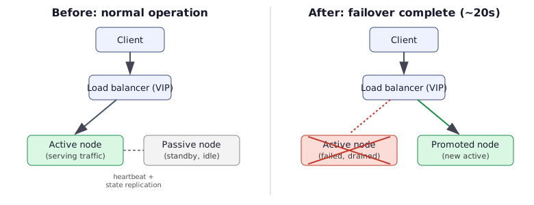
A Concrete Failover Timeline
The diagram above compresses a real sequence of events. A typical active-passive failover behind a health-checking load balancer looks like this:
- T+0s — the active node crashes (process dies, kernel panic, instance terminated). In-flight requests on open connections start failing or hanging.
- T+0s to T+10s — the load balancer's health checker polls the active node every 5 seconds and requires 2 consecutive failures before acting (a typical "unhealthy threshold: 2, interval: 5s" configuration). The first failed check lands somewhere in this window depending on timing.
- T+10s — the second consecutive health check fails, crossing the unhealthy threshold. The load balancer marks the active node unhealthy and stops routing new connections to it.
- T+10s to T+15s — an external orchestrator (or the standby itself, via a lost-heartbeat timeout) confirms the active node is actually down — not just slow — and triggers promotion of the passive standby. This step exists specifically to avoid a false failover on a single missed check.
- T+15s to T+20s — the standby finishes promotion: it replays any un-applied replicated writes, binds the virtual IP (VIP) or updates DNS/service-discovery records, and starts accepting traffic.
- T+~20s — the load balancer's next health check against the newly promoted node succeeds; new connections are routed to it. Total detection-to-recovery time: roughly 20 seconds.
Two numbers matter more than the total: detection time (health-check interval × unhealthy threshold) and promotion time (replaying replication lag, rebinding network identity). Tightening the health-check interval speeds up detection but raises the risk of false positives — flapping a healthy node in and out of service under transient load. That's a real trade-off, not a free dial to turn down.
Why Those Seconds Are the Availability Lever: MTBF and MTTR
The nines above and the timeline here are the same quantity viewed twice, and one identity connects them:
Availability = MTBF / (MTBF + MTTR) — where MTBF is mean time between failures (how rarely it breaks) and MTTR is mean time to recovery (how fast it comes back).
Assume a node that fails once a month — MTBF = 30 days = 2,592,000 seconds (an assumption, chosen to make the arithmetic legible). Vary only the recovery time:
- With the automated 20-second failover traced above: 2,592,000 / (2,592,000 + 20) ≈ 99.99923% — about 4 minutes of downtime per year.
- With manual recovery, 4 hours (page someone, they log in, they promote by hand): 2,592,000 / (2,592,000 + 14,400) ≈ 99.45% — about 48 hours per year.
Same hardware, same failure rate, roughly 720× more downtime — because 4 hours is 720 × 20 seconds. Halving MTTR buys exactly as much availability as doubling MTBF, and MTTR is the one you can actually engineer: you cannot make a disk fail less often, but you can make its replacement take seconds instead of hours. Redundancy plus automated failover is an attack on MTTR — the spare unit exists so that recovery is a promotion rather than a repair. That is why the detection and promotion numbers in the timeline above are the real availability levers, and why identical hardware can deliver two nines or five depending entirely on recovery automation.
Redundancy Models: N+1, N+M, 2N, 2N+1
"N" is the number of units actually required to carry the load. The redundancy model describes how many extra units are provisioned on top of N, and therefore how many simultaneous failures the system can absorb.
| Model | Meaning | Simultaneous failures tolerated | Extra capacity provisioned |
|---|---|---|---|
| N+1 | N units to carry load, plus exactly 1 spare | 1, regardless of how large N is | 1/N extra (shrinks as N grows) |
| N+M | N units to carry load, plus M spares | M | M/N extra |
| 2N | Every unit fully duplicated — two independent, complete N-unit stacks | Loss of one entire stack at once, if correlated | 100% extra |
| 2N+1 | 2N plus one additional spare unit | One entire stack plus one more independent failure | 100%+ extra |
N+1 is capacity-efficient but only ever tolerates a single failure at a time — it assumes failures are independent and rare enough that a second won't arrive before the first is repaired. N+M generalizes this to tolerate M concurrent failures, at the cost of M/N extra capacity sitting mostly idle. 2N is the model used when failures are expected to be correlated — an entire rack, availability zone, or data center going down together — because it guarantees a fully independent second stack rather than scattered spares. 2N+1 adds one more unit on top of that so that even after losing a whole redundant stack, the survivor can still tolerate one additional independent failure.
Why load redistribution, not just "did it survive," is the real question
Tolerating a failure and surviving it un-degraded are different claims. Take three application nodes behind a load balancer, each intentionally kept at 70% utilization exactly so there's headroom for a failure:
Total demand = 3 nodes × 70% = 210% of one node's capacity. If one node fails, the remaining 2 nodes must absorb all 210% of that demand: 210% ÷ 2 = 105% per surviving node — an overload, not graceful degradation.
The general formula for N identical nodes each running at utilization U, after losing one node: new utilization = U × N ÷ (N − 1). This bites hardest at small N — a 2-node "N+1" pair running at 70% each becomes 140% on the survivor, a full outage rather than a slowdown. The fix is either running at lower baseline utilization (headroom sized for N−1, not N), or provisioning enough spares (N+M or 2N) that losing one unit doesn't hand its full share to the rest.
Choosing a Redundancy Strategy
Active-active vs. active-passive
Active-active: every redundant node serves live traffic simultaneously — this is what the N+1/N+M capacity math above assumes. Use it when the workload is stateless, or the state layer already handles concurrent writers (a properly replicated database, idempotent processing). It uses the hardware you're paying for fully, and failover is just "route around the dead one" — no promotion step, no promotion latency.
Active-passive: one node serves traffic; the standby stays idle (or serves only reads) and takes over on failure, as in the diagram above. Use it when the component holds state that cannot be safely written by two nodes at once without a coordination protocol — a single-writer database primary, a distributed lock service leader. The cost is real: the standby's capacity sits unused during normal operation, and every failover pays the detection-plus-promotion latency traced above.
When not to use active-passive: if the workload can tolerate active-active's coordination requirements (stateless services, queues with idempotent consumers, read-heavy caches), defaulting to active-passive wastes half the fleet's capacity for no availability benefit — active-active gives the same failure tolerance without the idle standby or the failover pause.
N+1 vs. 2N
Reach for N+1 or N+M when failures are independent and uncorrelated — individual disks, individual server processes, individual NICs — and capacity efficiency matters, since the spare-to-load ratio shrinks as N grows. Reach for 2N (or 2N+1) when failures are correlated at a larger blast radius — a rack losing power, an availability zone losing network, a whole data center — because N+1's single spare, if it lives in the same failure domain as the N units, fails along with them and buys nothing. The trade-off is cost: 2N is a flat 100%+ capacity tax versus N+1's 1/N tax, so 2N is usually reserved for the tiers where an outage is unacceptable (payment processing, the control plane itself), not applied uniformly across the whole system.
Redundancy vs. replication
Use replication specifically to make a stateful component redundant — it's a mechanism, not a substitute goal. Don't stop at "the database is replicated" and call the system redundant: replication typically covers one component, the data tier. Everything else in the request path — load balancer, DNS, network path, the application tier itself, power — needs its own redundancy strategy, chosen independently, or it becomes the uncapped single point of failure the LB-in-series example above illustrated. The trade-off with replication specifically is consistency: synchronous replication (needed for a standby to be immediately promotable with zero data loss) adds write latency and can block writes if a replica is unreachable, while asynchronous replication avoids that latency cost by accepting a data-loss window (replication lag) if the primary fails before a write propagates.
Takeaways
- Redundancy removes single points of failure by duplicating critical components; replication is one mechanism for making stateful components redundant, not a synonym for the whole practice.
- Parallel components multiply away unavailability; series components multiply away availability. Every non-redundant component in the request path becomes the ceiling on the whole system's uptime, no matter how redundant everything else is — three six-nines app servers behind one non-redundant, four-nines-adjacent load balancer still cap out around four nines.
- Failover isn't instantaneous: detection time (health-check interval × unhealthy threshold) plus promotion time (replication catch-up, VIP/DNS rebind) both count, and tightening detection too aggressively trades false-positive flapping for faster recovery.
- N+1 tolerates exactly one failure regardless of scale and gets cheaper per unit as N grows; N+M generalizes to M concurrent failures; 2N and 2N+1 exist for correlated failure domains — racks, zones, data centers — where a single spare in the same blast radius buys nothing.
- Surviving a failure and surviving it un-degraded are different claims — after losing 1 of N nodes each at utilization U, survivors jump to U×N/(N−1); headroom has to be sized for N−1 nodes, not N.
- Pick active-active when the state layer tolerates concurrent writers, for full capacity utilization and no-promotion failover; pick active-passive only when a single-writer invariant forces it, and budget for the idle standby and the failover latency it costs.
Sources
- Google, Site Reliability Engineering (O'Reilly, 2016) — availability math, redundancy models, and failover mechanics.
- AWS Well-Architected Framework, Reliability Pillar — "design for redundancy" and workload distribution best practices.
- Google Cloud Architecture Framework, Reliability category — N+1/2N redundancy guidance for infrastructure design.
- Original site lesson: What is Redundancy, site/system-design/redundancy/001-what-is-redundancy.html.
🤖 Don't fully get this? Learn it with Claude
Stuck on What is Redundancy? Open Claude, copy a block below, and it'll teach you this exact concept — visually and interactively.
Build the mental picture, not memorization.
I just read a lesson on **What is Redundancy** (System Design) and want to truly understand it. Explain What is Redundancy from first principles using ONE vivid real-world analogy and a visual mental model — draw it as ASCII art or a clear step-by-step diagram — with a concrete example using real numbers. Then ask me one question to check I got the mental picture, and wait for my reply. If you're unsure or a claim isn't standard, say so and reason from first principles instead of guessing.
Socratic — adapts to where you're stuck.
Teach me **What is Redundancy** interactively. Ask me ONE guiding question at a time, wait for my answer, and adapt to my confusion — build the idea with me step by step instead of explaining it all at once. If you're unsure or a claim isn't standard, say so and reason from first principles instead of guessing.
Active recall exposes what you missed.
Quiz me on **What is Redundancy** with 5 questions, easy to tricky, ONE at a time. Tell me if each answer is right; at the end, explain clearly what I got wrong and why. If you're unsure or a claim isn't standard, say so and reason from first principles instead of guessing.
Intuition + hook + flashcards for long-term memory.
Help me remember **What is Redundancy** for the long term: give the one-sentence intuition, a memorable hook/mnemonic, a tiny worked example, and 3 active-recall flashcards (Q -> A). If you're unsure or a claim isn't standard, say so and reason from first principles instead of guessing.