Native Table Partitioning — Pruning, Local Indexes & Detach-for-Retention
Native table partitioning works because one logical table is physically stored as a set of smaller child tables (partitions), each holding a disjoint slice of the rows chosen by a partition key. The database keeps the routing rule — each partition's bound — in its catalog. An INSERT is routed to the one child whose bound covers its key; and, the payoff, a SELECT whose WHERE clause constrains the partition key lets the planner delete whole child tables from the plan before a single row is read. You turn "scan a billion rows and filter" into "scan the one 80-million-row child that could possibly match."
This is a single-node, database-layer technique, and that distinction is the whole reason to reach for it rather than sharding. Every partition of orders lives in the same PostgreSQL or MySQL instance, on the same disks, under one transaction manager. Partitioning changes the physical layout and the planner's search space inside one node; it buys you pruning, cheap bulk retention, and smaller indexes — not more CPU, RAM, or IOPS. Application-level sharding (splitting rows across many independent database nodes) is the different tool for when one node is out of headroom. The two compose — a sharded fleet where each shard also partitions its big tables by time is common — but do not confuse them: partitioning never adds a machine.
Declarative partitioning: RANGE, LIST, HASH
"Declarative" means you state the partitioning scheme on the parent and the engine owns routing and pruning — you don't hand-write triggers or UNION ALL views (the old "partitioning by convention" that PostgreSQL replaced in v10, and that MySQL never needed). Three strategies cover essentially everything:
- RANGE — contiguous, ordered key ranges. The canonical choice for time-series (one partition per day/month) and any monotonically growing key. Bounds are half-open in PostgreSQL:
FROMinclusive,TOexclusive. - LIST — explicit sets of discrete values. Good for low-cardinality categoricals:
region,tenant_tier,country. - HASH — the engine hashes the key into N buckets by modulus. Use it to spread write/heat evenly when there is no natural range or list — e.g. partition by
user_idso no single partition is a hotspot. HASH gives even distribution but loses range pruning (a date range can't prune a hash ofuser_id).
PostgreSQL — a monthly RANGE-partitioned orders:
CREATE TABLE orders (
    id           bigint GENERATED ALWAYS AS IDENTITY,
    order_date   date   NOT NULL,
    customer_id  bigint NOT NULL,
    amount_cents bigint NOT NULL,
    PRIMARY KEY (id, order_date)          -- PK MUST include the partition key (see below)
) PARTITION BY RANGE (order_date);

CREATE TABLE orders_2025_01 PARTITION OF orders
    FOR VALUES FROM ('2025-01-01') TO ('2025-02-01');   -- Feb 1 belongs to the NEXT partition
CREATE TABLE orders_2025_02 PARTITION OF orders
    FOR VALUES FROM ('2025-02-01') TO ('2025-03-01');
-- ... one per month ...
CREATE TABLE orders_default PARTITION OF orders DEFAULT;  -- catch rows that fit no bound
LIST and HASH on the same engine:
-- LIST: route by region
CREATE TABLE events (id bigint, region text NOT NULL, payload jsonb)
    PARTITION BY LIST (region);
CREATE TABLE events_us PARTITION OF events FOR VALUES IN ('us-east','us-west');
CREATE TABLE events_eu PARTITION OF events FOR VALUES IN ('eu-west','eu-central');

-- HASH: spread user_id evenly over 4 buckets
CREATE TABLE sessions (user_id bigint NOT NULL, started_at timestamptz)
    PARTITION BY HASH (user_id);
CREATE TABLE sessions_0 PARTITION OF sessions FOR VALUES WITH (MODULUS 4, REMAINDER 0);
CREATE TABLE sessions_1 PARTITION OF sessions FOR VALUES WITH (MODULUS 4, REMAINDER 1);
CREATE TABLE sessions_2 PARTITION OF sessions FOR VALUES WITH (MODULUS 4, REMAINDER 2);
CREATE TABLE sessions_3 PARTITION OF sessions FOR VALUES WITH (MODULUS 4, REMAINDER 3);
MySQL/InnoDB expresses the same idea inline on one statement (partitions are declared in the CREATE TABLE). RANGE COLUMNS compares the raw column so you avoid the old TO_DAYS() wrapper:
CREATE TABLE orders (
    id           BIGINT NOT NULL AUTO_INCREMENT,
    order_date   DATE   NOT NULL,
    amount_cents BIGINT NOT NULL,
    PRIMARY KEY (id, order_date)          -- MySQL: every UNIQUE/PK key must include the partition column
)
PARTITION BY RANGE COLUMNS (order_date) (
    PARTITION p2025_01 VALUES LESS THAN ('2025-02-01'),
    PARTITION p2025_02 VALUES LESS THAN ('2025-03-01'),
    PARTITION pmax     VALUES LESS THAN (MAXVALUE)      -- safety catch-all
);
Partition pruning in the planner — the payoff, on an EXPLAIN
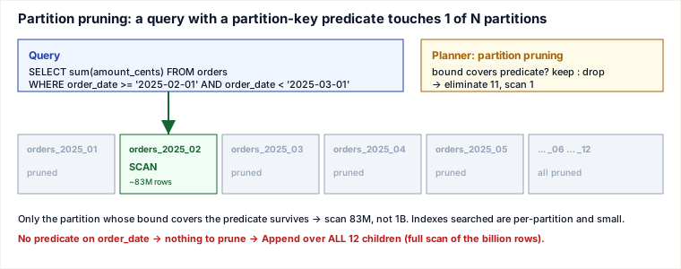
Pruning is the planner proving, from the query's predicates and the partition bounds in the catalog, that a partition cannot contain a matching row, and dropping it from the plan. In PostgreSQL enable_partition_pruning is on by default. Watch what a partition-key predicate does to the plan — only one child appears:
EXPLAIN
SELECT sum(amount_cents) FROM orders
WHERE  order_date >= '2025-02-01' AND order_date < '2025-03-01';

 Aggregate
   ->  Seq Scan on orders_2025_02 orders     -- ONLY February; all other months pruned
         Filter: (order_date >= '2025-02-01' AND order_date < '2025-03-01')
Drop the predicate and the planner has nothing to prune with — it builds an Append over every child:
EXPLAIN SELECT sum(amount_cents) FROM orders;

 Aggregate
   ->  Append
         ->  Seq Scan on orders_2025_01 orders_1
         ->  Seq Scan on orders_2025_02 orders_2
         ->  Seq Scan on orders_2025_03 orders_3
         ...                                   -- all 12 partitions scanned
Two flavors matter. Plan-time pruning happens when the bound is a constant literal (above). Run-time pruning handles a value not known until execution — a bind parameter or the output of a subplan — and shows as (never executed) on the skipped children or a Subplans Removed: N line under the Append. This is why a prepared statement with order_date = $1 still prunes at execution even though the plan was built generically.
Partition-wise joins and aggregates
Pruning helps a single table; partition-wise operations help when two large tables are partitioned the same way, or when you aggregate by the partition key. If orders and order_items are both RANGE-partitioned on order_date with matching bounds, PostgreSQL can join them partition-by-partition — January-orders ⋈ January-items, February ⋈ February — instead of joining the two giant tables whole. Each sub-join works on a slice that fits in memory, hashes are smaller, and the sub-joins parallelize. This is off by default; enable it:
SET enable_partitionwise_join = on;        -- join matching partitions pairwise
SET enable_partitionwise_aggregate = on;   -- push GROUP BY down per partition
Partition-wise aggregate is the twin: GROUP BY order_date (or any key that can't span partitions) is computed inside each partition and the partial results combined, rather than funneling every row through one grouping node. Both are off by default because they raise planning cost and memory on tables with many partitions — turn them on for the specific analytical queries that benefit.
Local vs global indexes, and the unique-constraint gotcha
This is the concept interviewers probe, because it silently constrains your schema. PostgreSQL indexes on a partitioned table are always local — physically there is no single B-tree spanning the whole table; an index "on the parent" is a template that materializes as one independent index per partition. Creating it cascades to every child (and to future children):
CREATE INDEX ON orders (customer_id); -- becomes a separate btree in EACH partitionThe direct consequence: a UNIQUE constraint or PRIMARY KEY must include every partition-key column. With only local indexes, PostgreSQL can enforce uniqueness within each partition but has no structure that sees across partitions — so it cannot promise a bare id is globally unique unless id is itself the partition key. That is exactly why the orders PK above is (id, order_date), not (id): uniqueness is enforced per-month, and the partition key rides along so the engine can route and check within one child. MySQL enforces the identical rule ("every unique key must use all columns of the partitioning expression").
Contrast Oracle, which supports true GLOBAL indexes — one B-tree over all partitions that can enforce a global unique key on a non-partition column. The price is that dropping a partition invalidates or forces a maintenance rebuild of every global index (UPDATE INDEXES), which reintroduces exactly the expensive, blocking work that local indexes let you skip. PostgreSQL/MySQL deliberately trade away global uniqueness on arbitrary columns to keep partition drop/attach as pure metadata.
To build partition indexes without a long lock, combine with the online-schema discipline: build the index CONCURRENTLY on each existing partition first, create the index ON ONLY the parent, then ALTER INDEX ... ATTACH PARTITION to mark the parent index complete — so writes keep flowing throughout, just as with any large index build.
ATTACH / DETACH — retention as a metadata operation
The operational jackpot. To drop a month of data with a plain table you run DELETE FROM orders WHERE order_date < '2024-02-01' — which reads and marks tens of millions of rows dead, floods the WAL/binlog, leaves the table bloated until autovacuum/purge catches up, and ships every deletion to replicas as lag. With partitioning, dropping the oldest month is a catalog edit: detach the partition and drop the now-standalone table.
-- PostgreSQL retention: remove Jan-2024 instantly, no row-by-row DELETE
ALTER TABLE orders DETACH PARTITION orders_2024_01;   -- metadata: child becomes a normal table
DROP TABLE orders_2024_01;                             -- frees the files in one step
-- (PG14+: DETACH PARTITION ... CONCURRENTLY avoids the brief ACCESS EXCLUSIVE lock)

-- MySQL equivalent, also metadata-only:
ALTER TABLE orders DROP PARTITION p2024_01;
The reverse, ATTACH, adds next month's partition. Do it cheaply by giving the incoming table a CHECK that already matches the target bound — then ATTACH trusts the constraint and skips the full validation scan it would otherwise run to prove every row fits:
CREATE TABLE orders_2025_03 (LIKE orders INCLUDING DEFAULTS INCLUDING CONSTRAINTS INCLUDING INDEXES);
-- INCLUDING INDEXES is essential: it builds the local index matching the parent's
-- partitioned PRIMARY KEY up front, so ATTACH is metadata-only. Omit it and ATTACH must
-- build that index during the operation — an O(rows) scan, not the cheap swap you wanted.
-- pre-load / build indexes on this standalone table off the hot path, then:
ALTER TABLE orders_2025_03
    ADD CONSTRAINT ck CHECK (order_date >= '2025-03-01' AND order_date < '2025-04-01');
ALTER TABLE orders ATTACH PARTITION orders_2025_03
    FOR VALUES FROM ('2025-03-01') TO ('2025-04-01');   -- matching CHECK → no scan
Automate this so a partition always exists ahead of the clock (e.g. pg_partman, or a cron that pre-creates next month). A missing partition means inserts hit the DEFAULT partition or, if there is none, fail.
Worked example: a 1-billion-row time-series orders table
Twelve monthly RANGE partitions, ~83M rows each, ~1B total, one PostgreSQL node. Trace the two operations that justify the whole design.
1) A date-ranged query prunes to one partition. The dashboard query "revenue for February 2025":
SELECT sum(amount_cents) FROM orders
WHERE  order_date >= '2025-02-01' AND order_date < '2025-03-01';
The planner reads the catalog bounds, proves only orders_2025_02 can match, and scans that one 83M-row child using its small local index — the other eleven partitions and their indexes are never opened. Work done: ~1/12th of the table. On one un-partitioned billion-row table the same query walks a single enormous index (or seq-scans 1B rows), and that index is ~12× taller/larger so each lookup touches more pages and the buffer cache holds proportionally less of it.
2) Retention drops last year's data instantly. Policy: keep 12 months. When March 2025 opens, February 2024 ages out:
ALTER TABLE orders DETACH PARTITION orders_2024_02;
DROP TABLE orders_2024_02;         -- ~83M rows gone in milliseconds, metadata + file unlink
Compare the plain-table path: DELETE FROM orders WHERE order_date < '2024-03-01' would read and tombstone ~83M rows in one shot — minutes of I/O, a WAL flood, 83M dead tuples pinning the vacuum horizon and bloating the table, and replicas lagging while they replay every delete. The partitioned version does zero row work. This asymmetry — O(1) metadata vs O(rows) scan-and-bloat — is the single strongest argument for partitioning a large append-and-expire table.
Pitfalls
- No partition key in the query → every partition is scanned.
WHERE customer_id = 42on a table partitioned byorder_datecannot prune — the planner mustAppendover all N children and search N separate indexes. This is often slower than one big table's single index. Mitigate by including the partition key when you can (AND order_date >= ...), or partition by the column your hot queries actually filter on. Choosing the partition key is choosing which queries get to prune. - Too many partitions → planner and lock overhead. Every partition is a relation the planner must consider and lock. Thousands-to-tens-of-thousands of partitions inflate planning time and per-query memory, and can exhaust
max_locks_per_transaction. Prefer partitions in the hundreds; if daily partitions would give you 3,650 over ten years, use monthly plus retention. Sub-partitioning multiplies the count — use it sparingly. - Unique constraints must include the partition key (above) — you cannot enforce global uniqueness on a natural key like
emailunless it is the partition key. Model around this early; retrofitting is painful. - Cross-partition
ORDER BY/LIMITand updates that move the key. An ordered query spanning partitions needs a merge/sort across children (anAppend, not aMerge Append, unless each child is pre-sorted). And anUPDATEthat changes a row's partition key is physically aDELETE+INSERTacross children — correct in modern PostgreSQL/MySQL but not free. - A missing future partition rejects inserts (or dumps them in
DEFAULT). Always provision partitions ahead of time and monitor.
Trade-off: native partitioning vs application sharding vs one big table
These answer different questions. One big table asks nothing of you and is correct until it isn't. Native partitioning solves manageability and pruning within one node. Application sharding solves capacity beyond one node — and only that, at real cost.
| Dimension | One big table | Native partitioning (1 node) | Application sharding (N nodes) |
|---|---|---|---|
| What it buys | Simplicity | Pruning, small per-partition indexes, O(1) bulk retention | More CPU / RAM / IOPS / disk — horizontal scale |
| Scales writes/storage past one machine? | No | No — same node, same limits | Yes — that's the point |
| Cross-cutting queries & joins | Trivial | Trivial (one node, one planner) | Hard — scatter-gather, cross-shard joins app-side |
| Transactions across the key space | ACID, free | ACID, free | Distributed txns / 2PC or give them up |
| Global unique / FK on any column | Yes | Only if it includes the partition key | No global guarantee across shards |
| Retention of old data | Mass DELETE (bloat, lag) | DETACH+DROP, metadata-only | Per-shard, same partitioning trick inside each |
| Operational cost | Lowest | Low (one node to run) | High — rebalancing, routing, ops of N nodes |
When each: Start with one big table — don't partition on speculation; pruning needs the right key and adds planning overhead, so an unpartitioned table with a good index often wins until you're in the hundreds-of-millions of rows or you have a real retention/archival need. Move to native partitioning when a single large table on a node you're not outgrowing has a natural slicing key (almost always time) and you want cheap retention, smaller indexes, and pruning for range queries — you stay fully ACID and keep easy joins. Reach for application sharding only when one node genuinely can't hold the write throughput or data volume; accept that you're trading away cross-key transactions, easy joins, and global constraints for capacity. And combine them at the top end: shard by tenant/user across nodes, and within each shard partition the big time-series tables by month.
Takeaways
- Partitioning is a single-node, planner-level layout, not scale-out. It gives you pruning, small per-partition indexes, and metadata-cheap retention on one machine; sharding is the separate tool for when you need more machines. They compose but solve different problems.
- Pruning only fires when the query constrains the partition key. Read it off
EXPLAIN(one child vs anAppendover all). Choose the partition key to match your hot filter — time for time-series — because a query without that predicate scans every partition and can be slower than one big indexed table. - Indexes are local, so unique keys must include the partition key. There is no global B-tree in PostgreSQL/MySQL; that's the deliberate trade that makes ATTACH/DETACH pure metadata (unlike Oracle's global indexes, which must rebuild on partition drop).
- DETACH+DROP is the killer feature: aging out a month is O(1) metadata versus an O(rows) mass
DELETEthat bloats and lags. Pre-create future partitions and build/attach indexes with the online-schema discipline so nothing blocks live traffic.
Sources
- PostgreSQL documentation — Table Partitioning (declarative RANGE/LIST/HASH, partition pruning, partition-wise join/aggregate GUCs, ATTACH/DETACH, DETACH CONCURRENTLY) and CREATE TABLE ... PARTITION OF.
- MySQL Reference Manual — Partitioning chapter: RANGE/LIST/HASH/COLUMNS, the rule that every unique key must include the partitioning columns, and
ALTER TABLE ... DROP/REORGANIZE PARTITION. - Oracle Database VLDB and Partitioning Guide — LOCAL vs GLOBAL partitioned indexes and index maintenance on partition operations (
UPDATE INDEXES), for the contrast. - pg_partman documentation — automated time/serial partition provisioning and retention.
- Kleppmann, Designing Data-Intensive Applications, ch. 6 (Partitioning) — partitioning vs. replication vs. sharding, secondary-index-by-document vs. by-term, and rebalancing trade-offs.
🤖 Don't fully get this? Learn it with Claude
Stuck on Native Table Partitioning — Pruning, Local Indexes & Detach-for-Retention? Open Claude, copy a block below, and it'll teach you this exact concept — visually and interactively.
Build the mental picture, not memorization.
I just read a lesson on **Native Table Partitioning — Pruning, Local Indexes & Detach-for-Retention** (Databases) and want to truly understand it. Explain Native Table Partitioning — Pruning, Local Indexes & Detach-for-Retention from first principles using ONE vivid real-world analogy and a visual mental model — draw it as ASCII art or a clear step-by-step diagram — with a concrete example using real numbers. Then ask me one question to check I got the mental picture, and wait for my reply. If you're unsure or a claim isn't standard, say so and reason from first principles instead of guessing.
Socratic — adapts to where you're stuck.
Teach me **Native Table Partitioning — Pruning, Local Indexes & Detach-for-Retention** interactively. Ask me ONE guiding question at a time, wait for my answer, and adapt to my confusion — build the idea with me step by step instead of explaining it all at once. If you're unsure or a claim isn't standard, say so and reason from first principles instead of guessing.
Active recall exposes what you missed.
Quiz me on **Native Table Partitioning — Pruning, Local Indexes & Detach-for-Retention** with 5 questions, easy to tricky, ONE at a time. Tell me if each answer is right; at the end, explain clearly what I got wrong and why. If you're unsure or a claim isn't standard, say so and reason from first principles instead of guessing.
Intuition + hook + flashcards for long-term memory.
Help me remember **Native Table Partitioning — Pruning, Local Indexes & Detach-for-Retention** for the long term: give the one-sentence intuition, a memorable hook/mnemonic, a tiny worked example, and 3 active-recall flashcards (Q -> A). If you're unsure or a claim isn't standard, say so and reason from first principles instead of guessing.