Indexing & Storage — Fanout Arithmetic, Optimizer Stats, Composite/Skip Scans & NULL/OR Pitfalls (Deep Dive)

A B+tree's depth is not a rule of thumb pulled from memory — it falls straight out of one division: how many (key, pointer) entries fit on a page. Get that division right and you can derive the depth of any index, for any key size, on the spot — instead of reciting “3–4 levels” and hoping the interviewer doesn't ask why.

This page assumes you already know the B+tree basics — internal vs leaf nodes, point lookup vs range scan, clustered vs secondary — covered in How Indexes Work and Indexes in Practice. It goes one level deeper into exactly the mechanisms an interviewer probes past the basics: the fanout arithmetic that makes depth re-derivable, why a busy table doesn't actually pay for every level on every lookup, how the optimizer decides selectivity in the first place, the composite-index rule and its real exception (skip scan), how insertion order fragments the tree, and the NULL/OR/NOT IN pitfalls that quietly break either correctness or index usage. The selectivity crossover arithmetic itself and the B-tree-vs-LSM storage-engine trade-off are covered in depth elsewhere in this guide — this page cross-references both rather than re-deriving them, and focuses on the indexing-specific angle: the structure itself, not the storage engine or the query planner's cost model in general.

1. Fanout arithmetic: deriving depth instead of memorizing it

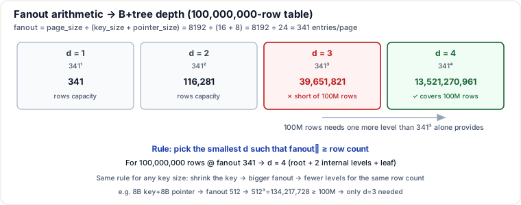
Every internal (routing) page in a B+tree holds a fixed number of (key, pointer) entries — the page's fanout. That number is just page capacity divided by entry size:

fanout = page_size ÷ (key_size + pointer_size)

Take a typical 8 KB page, a 16-byte key (e.g. a UUID stored as raw binary, or two 8-byte columns), and an 8-byte child pointer:

fanout = 8192 ÷ (16 + 8) = 8192 ÷ 24 ≈ 341 entries per page

Depth follows directly: a tree of depth d can address up to fanoutᴸ rows (root at the top, d−1 internal levels, leaf at the bottom). So the rule is: pick the smallest d such that fanoutᴸ ≥ row count.

Traced example: how many levels for 100,000,000 rows?

Depth d	Capacity = 341d	Covers 100M rows?
1	341	no
2	116,281	no
3	39,651,821 (≈39.65M)	no — short by more than half
4	13,521,270,961 (≈13.52B)	yes

341³ only reaches about 39.65 million — a 100-million-row table doesn't fit at depth 3, so it needs depth 4 (root + two internal levels + leaf). This is the arithmetic worth checking every time: a commonly repeated version of this example rounds straight to “100M rows ≈ depth 3” without checking that 341³ actually falls short of 100M — recompute it, don't recite it.

The same rule re-derives depth for any key size, because only the fanout changes:

Entry size (key+pointer)	Fanout (8KB page)	Depth for 100M rows
16 B (8B bigint key + 8B pointer)	8192÷16 = 512	5123 = 134,217,728 ≥ 100M ⇒ d = 3
24 B (16B key + 8B pointer)	8192÷24 ≈ 341	3413 ≈ 39.65M < 100M ⇒ d = 4
72 B (64B VARCHAR key + 8B pointer)	8192÷72 ≈ 113	1133 ≈ 1.44M < 100M ⇒ d = 4 (1134≈163M)

The qualitative takeaway a candidate should say out loud: narrower keys → higher fanout → the tree stays shallower for longer as the table grows. A bigint primary key needs one fewer level than a wide composite or text key at the same row count — which is exactly why "narrow, sequential primary keys" is standard schema-design advice, not folklore.

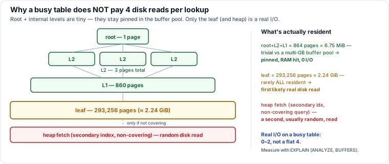
2. The buffer-pool caveat: a busy table does NOT pay 4 disk reads per lookup

The naive version of the fanout result — “depth 4 ⇒ 4 disk reads per lookup” — is wrong for any table that gets queried more than occasionally, because it silently assumes every page read is a cache miss. It isn't. The buffer pool (Postgres shared_buffers, InnoDB buffer pool) caches recently-touched pages in RAM, and the upper levels of a B+tree are the cheapest pages in the world to keep resident: they're tiny and they're touched by every single lookup, so they're the least likely pages to ever get evicted.

Continuing the 100M-row / fanout-341 example: the page counts per level work out to leaf ≈ 293,256 pages, one level up ≈ 860 pages, one level above that 3 pages, and a single root page — 864 pages total above the leaf, or exactly 6.75 MiB at 8 KB/page. That's a rounding error against a buffer pool that's typically gigabytes. In practice those 864 pages sit pinned in RAM permanently, and every lookup's root-to-just-above-leaf traversal costs zero real I/O. The leaf level, at ≈293,256 pages (≈2.24 GiB), is far too big to guarantee full residency — it's the first place a lookup can actually hit disk. And if the index is a secondary index, there's a further hop to the heap to fetch the row, which is usually the coldest, most random read of all.

So the corrected claim: on a warm, frequently-queried table, a lookup typically costs 0–2 real disk reads, not a flat 4 — 0 if everything relevant is hot, up to 2 if both the leaf page and the heap page happen to be cold. The “3–4 disk reads” number only describes a fully cold cache (e.g. right after a restart, or a table nobody has touched recently). Don't assume either number — measure it: EXPLAIN (ANALYZE, BUFFERS) in Postgres reports shared hit (buffer-pool hit, free) vs shared read (an actual I/O) per node.

3. Optimizer statistics: how the planner knows a predicate's selectivity in the first place

The Query Execution deep-dive on this guide derives the full selectivity-crossover arithmetic — the flat seq-scan cost vs. the linearly-growing index-scan cost, and the point where they cross. That page assumes the planner already has a selectivity number to plug into the formula. This section covers where that number actually comes from, because it's the part that breaks silently: the statistics.

ANALYZE (run automatically by autovacuum/autoanalyze, or by hand) samples the table and writes per-column entries into pg_statistic (exposed readably via pg_stats):

• n_distinct — an estimate of how many distinct values the column has.
• Most-common values (MCV list) — the top N most frequent values, each with its exact observed frequency.
• A histogram — the remaining (non-MCV) value range, split into roughly equi-depth buckets, so the planner can estimate how many rows fall into any range even without an exact frequency for that value.

The planner picks between two very different quality estimates depending on where the query's literal value falls:

• Value is in the MCV list — e.g. status = 'shipped' where 'shipped' is 91% of a 10M-row orders table and easily makes the MCV list — the planner uses that exact observed frequency. Selectivity estimate: spot-on.
• Value falls in a histogram bucket (not an MCV) — e.g. a rare, one-off value in a high-cardinality free-text column — the planner estimates using the bucket's average density (roughly (1 − ΣMCV freqs) / distinct values outside the MCV list), which is far less precise than an exact MCV frequency, especially if the true distribution inside that bucket is itself skewed.

Stale statistics is the failure mode that actually bites in production: after a large bulk load, bulk delete, or a sudden shift in value distribution, the MCV list and histogram still reflect the old data until the next ANALYZE runs. The planner then estimates selectivity from a distribution that no longer exists — which is exactly the "cardinality error propagates up the tree" failure mode the Query Execution page describes: one wrong leaf-level estimate feeds the cost formula of every join and sort above it, and can flip the chosen plan several levels up from where the real problem is.

4. Composite indexes: leftmost prefix, and the skip-scan exception

A composite index on (a, b) is physically sorted by a first, and only sorted by b within each distinct value of a. That's the mechanism behind the “leftmost prefix” rule: a predicate on a alone, or on (a, b) together, can seek directly, because a's ordering is global across the whole index. A predicate on b alone cannot — b's values are scattered inside every one of a's partitions, so there's no single contiguous range of the index to seek to. The textbook conclusion: (a, b) cannot serve WHERE b = ?.

That conclusion is the absolute reading, and it has a real, engine-supported exception: index skip scan (MySQL 8.0+, Oracle's “index skip scan”, and, natively, PostgreSQL 18+). The mechanism defeats the leftmost-prefix rule specifically when a has low cardinality:

1. The engine first finds the distinct values of a — cheap, because a is the leading, sorted column, so this is effectively a loose/distinct index scan, not a full pass over every row.
2. For each distinct value of a, it runs a normal, cheap range probe for b = ? within that a-partition — which is sargable again, because inside a fixed a, b really is locally sorted.
3. It unions the results across all of a's distinct values.

Traced example

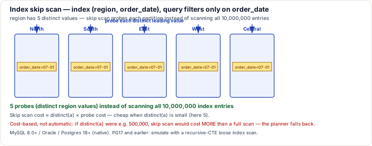
Table orders, 10,000,000 rows, index on (region, order_date). region has 5 distinct values. Query: WHERE order_date = '2026-07-01' — no predicate on region at all.

• Without skip scan: order_date is not the leading column, so (region, order_date) cannot be seeked on this predicate — the planner falls back to scanning the base table (or, in principle, the whole index, which is no cheaper). Either way, the access path touches on the order of every row in the table.
• With skip scan: the engine enumerates the 5 distinct region values, then does 5 probes — one per region — each a normal, cheap B-tree seek for order_date = '2026-07-01' inside that region's slice of the index.

5 probes vs. touching all 10,000,000 rows is the entire value proposition, and it only exists because distinct(region) = 5 is tiny. The cost model makes this explicit and bounded: skip-scan cost ≈ distinct(a) × probe cost. If region instead had, say, 500,000 distinct values, skip scan would issue 500,000 probes — almost certainly worse than a full scan — so the planner treats skip scan as one candidate plan among several and costs it like any other; it is never applied blindly. Note also that this is engine-specific: PostgreSQL 18 (GA September 2025) added native B-tree skip scan, automatically chosen by the planner when it's cost-effective — on PostgreSQL 17 and earlier, the closest workaround is a hand-written recursive-CTE “loose index scan” over the distinct leading values.

5. Insertion order and fragmentation: the index-specific angle

The Relational Model deep-dive on this guide already covers the UUIDv4-vs-monotonic primary-key trade-off from the key-design angle (natural vs. surrogate keys, InnoDB clustering). The index-specific mechanism underneath that recommendation is where a random key forces a page split. A B+tree keeps every leaf at the same depth by splitting a leaf in two the moment an insert overflows it, then pushing the new middle key up to the parent (which may split too). That's cheap and rare when inserts land at the rightmost leaf, because a leaf only needs to split when it's actually full — and an ever-increasing key (auto-increment, UUIDv7, ULID) always appends past the current maximum, so exactly one leaf (the rightmost one) ever fills up and splits, in order, one at a time.

A random key like UUIDv4 destroys that locality: each insert's key hashes to an essentially random position across the entire existing keyspace, so it can overflow any leaf, not just the rightmost one. At scale this means splits happen constantly, scattered across the whole tree, leaves end up roughly half-full on average (freshly split pages start half-empty), and pages that are logically adjacent by key order are physically scattered across disk — the opposite of the sequential-append pattern a storage engine is optimized for. The net effect: more pages for the same data (bloat), worse buffer-pool hit rate (adjacent keys aren't adjacent on disk, so a range scan or a warm working set needs more distinct pages resident to get the same hit rate), and more write amplification from constant splitting.

6. NULL, OR, NOT IN — three ways a predicate quietly breaks index use (or correctness)

• IS NULL can use an index. The common belief that “NULLs aren't indexed” is folklore, not mechanism — Postgres's B-tree indexes do store NULL entries (sorted, by default, after all non-NULL values), so WHERE col IS NULL is a normal, sargable index seek to that end of the index, not a full scan.
• OR across two different columns needs a bitmap union of two indexes. WHERE a = 5 OR b = 10, with separate single-column indexes on a and b, can't be served by either index alone in one probe — a single B-tree only orders by one column. But it doesn't have to fall back to a sequential scan either: the planner can build a bitmap of matching heap locations from the a index, a separate bitmap from the b index, OR the two bitmaps together (a BitmapOr), and then do one bitmap heap scan that visits each flagged page exactly once. Two single-column indexes can jointly serve an OR that neither can serve alone — the corresponding AND case uses a BitmapAnd (intersection) instead.
• NOT IN with a NULL-producing subquery is a correctness bug, not just a slow plan. WHERE col NOT IN (SELECT x FROM t2) expands under three-valued logic to col <> v1 AND col <> v2 AND … AND col <> NULL for every row returned by the subquery. If t2.x can be NULL, then col <> NULL evaluates to UNKNOWN for every row, which makes the entire AND chain UNKNOWN (never TRUE) — so the query silently returns zero rows, regardless of what actually doesn't match v1/v2. It also can't use an index the way a correlated check could. The fix is NOT EXISTS (SELECT 1 FROM t2 WHERE t2.x = col), which handles NULLs correctly and can still drive an index lookup per outer row.
• An index-only scan still isn't guaranteed to skip the heap. Postgres's index-only scan avoids the heap only for rows on a page the visibility map marks “all-visible” (every tuple on that page is visible to every current transaction — i.e., nothing on it has been recently inserted, updated, or deleted and not yet vacuumed). For a page whose visibility-map bit is unset — typically a page with recent writes — Postgres still has to visit the heap tuple to check MVCC visibility, because the index itself carries no visibility information. So “index-only” is a best-case label, not a guarantee: a table with a hot, frequently-modified working set gets fewer of index-only scan's benefits until VACUUM catches those pages up.

Pitfalls a working engineer actually hits

• Quoting “3–4 disk reads” for a hot table. That number describes a cold cache; on a busy table the real number is usually 0–2 — verify with EXPLAIN (ANALYZE, BUFFERS), don't assume either direction.
• Assuming (a, b) can never help a query on b alone — missing the skip-scan escape hatch when a is low-cardinality, and equally, assuming skip scan always helps when a's cardinality later grows into the thousands or millions (it doesn't — it's cost-based and can lose badly).
• Bulk-loading or bulk-deleting without a follow-up ANALYZE. The MCV list and histogram still reflect the old distribution until the next analyze runs, so the very next query can get a confidently wrong selectivity estimate and a bad plan.
• Rewriting col IS NULL into a workaround (e.g. COALESCE(col, 'sentinel') = 'sentinel') in the mistaken belief that NULLs aren't indexed — the rewrite actually breaks sargability that the plain IS NULL already had.
• Using NOT IN against a subquery that can produce a NULL — a silent empty result set, not an error, so it can ship unnoticed until someone asks why a row that should be excluded/included isn't.
• Assuming a covering index means zero heap I/O. A recently-written hot table can still force heap fetches during an "index-only" scan until the visibility map catches up behind autovacuum.
• A random UUIDv4 primary key looking fine in a small dev table (it all fits in RAM) but fragmenting badly once the table is large enough that splits and cache misses actually cost something — the damage is invisible until scale exposes it.

Judgment layer: how a senior engineer decides

• Will a composite index help this query? Predicate matches the leftmost prefix of (a, b, …), or the full tuple → full, direct benefit. Predicate skips the leading column but that column is low-cardinality (a handful to low hundreds of distinct values) → skip scan may still rescue it on engines that support it (MySQL 8+/Oracle), but verify it's actually chosen — don't assume. Leading column skipped and high-cardinality → skip scan will lose to a full scan; add a proper index with the queried column leading instead.
• Monotonic vs. random primary key. Monotonic (auto-increment/UUIDv7/ULID) keeps inserts appending to the rightmost leaf — dense pages, predictable splits, good cache locality — at the cost of concentrating insert traffic on one hot page under very high concurrency. Random (UUIDv4) spreads writes across the whole tree — which can relieve that single-page insert hotspot in some very high-throughput/sharded designs — but pays for it with page-split churn, bloat, and worse cache locality everywhere else. Default to monotonic; only reach for random keys when a specific, measured hot-page contention problem justifies the fragmentation trade-off.
• Trusting stale-looking statistics. If a plan looks wrong right after a large load/delete/schema change, check pg_stats and re-run ANALYZE before reaching for a query rewrite or an index hint — a stale MCV/histogram, not a missing index, is the more common root cause.

Takeaways

• Fanout = page_size ÷ (key_size + pointer_size); depth is the smallest d with fanout^d ≥ row count — recompute it for any key size instead of reciting “3–4 levels.”
• Only the leaf (and, for a secondary index, the heap) is a likely real disk read on a busy table — root and internal levels are trivially small and stay pinned in the buffer pool.
• Selectivity comes from pg_statistic's MCV list and histogram, not from the index itself — stale stats break a plan even with a perfect index in place.
• “Absolute” index rules bend under real mechanisms: skip scan can serve a query on a composite index's trailing column, BitmapOr lets two single-column indexes jointly serve an OR, and Postgres does index NULLs — but NOT IN with a NULL-producing subquery and a non-all-visible heap page both still bite.

---

Re-authored/Deepened for this guide.

I just read a lesson on **Indexing & Storage — Fanout Arithmetic, Optimizer Stats, Composite/Skip Scans & NULL/OR Pitfalls (Deep Dive)** (Databases) and want to truly understand it. Explain Indexing & Storage — Fanout Arithmetic, Optimizer Stats, Composite/Skip Scans & NULL/OR Pitfalls (Deep Dive) from first principles using ONE vivid real-world analogy and a visual mental model — draw it as ASCII art or a clear step-by-step diagram — with a concrete example using real numbers. Then ask me one question to check I got the mental picture, and wait for my reply. If you're unsure or a claim isn't standard, say so and reason from first principles instead of guessing.

Teach me **Indexing & Storage — Fanout Arithmetic, Optimizer Stats, Composite/Skip Scans & NULL/OR Pitfalls (Deep Dive)** interactively. Ask me ONE guiding question at a time, wait for my answer, and adapt to my confusion — build the idea with me step by step instead of explaining it all at once. If you're unsure or a claim isn't standard, say so and reason from first principles instead of guessing.

Quiz me on **Indexing & Storage — Fanout Arithmetic, Optimizer Stats, Composite/Skip Scans & NULL/OR Pitfalls (Deep Dive)** with 5 questions, easy to tricky, ONE at a time. Tell me if each answer is right; at the end, explain clearly what I got wrong and why. If you're unsure or a claim isn't standard, say so and reason from first principles instead of guessing.

Help me remember **Indexing & Storage — Fanout Arithmetic, Optimizer Stats, Composite/Skip Scans & NULL/OR Pitfalls (Deep Dive)** for the long term: give the one-sentence intuition, a memorable hook/mnemonic, a tiny worked example, and 3 active-recall flashcards (Q -> A). If you're unsure or a claim isn't standard, say so and reason from first principles instead of guessing.