Query Execution — Selectivity, the Cost Model, Join Algorithms, Spills & Sargability (Deep Dive)
The single most common query-execution interview question is “there’s an index on that column — why did the planner run a sequential scan anyway?” The one-line mechanism: an index match costs one random heap-page fetch, while a sequential scan pays for pages in the cheapest possible order — one linear pass, heavily prefetched. So once a predicate matches more than a small slice of the table, paying for many scattered single-row fetches costs more in total than just reading every page once. Above that crossover point, the seq scan is the objectively cheaper plan, not a planner mistake.
This page assumes you already know the iterator model (operators pull rows from their children one at a time) and that EXPLAIN prints a cost. Here we go one level deeper into the arithmetic and mechanisms an interviewer actually probes: selectivity, the cost model’s startup/total split, why join algorithms are constrained by predicate shape, what a hash join does when it can’t fit in memory, how to write predicates an index can actually use, and three failure modes that hide inside a single EXPLAIN line.
Selectivity: why the planner sometimes ignores your index
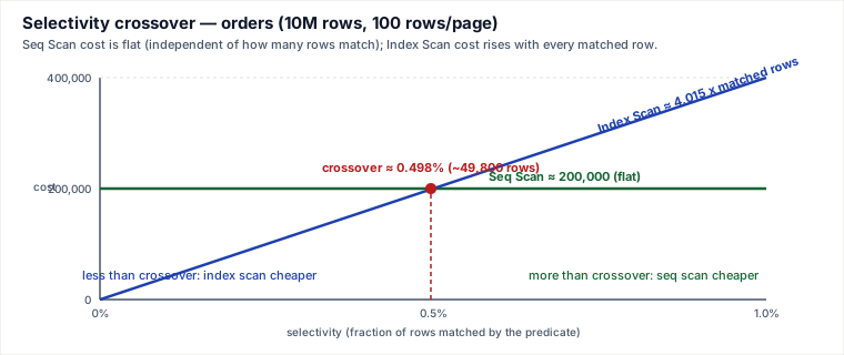
Selectivity is the fraction of a table’s rows a predicate matches. It is the single number that decides between an index scan and a sequential scan, because the two access paths have completely different cost shapes:
- A sequential scan reads every page of the table once, in physical order. Its cost is flat — it does not care how many rows match the predicate, because it visits every page regardless to check.
- An index scan pays a small cost to descend the B-tree, then for every matching row does a heap fetch to retrieve the actual row — and in the worst case (no correlation between index order and physical row order) that heap fetch lands on a different, essentially random, page almost every time. Cost grows linearly with the number of matches.
A flat line and a rising line cross exactly once. Below the crossover the index wins; above it the seq scan wins — and a plan that “ignores your index” is usually doing the arithmetic correctly.
Traced example
Table orders: 10,000,000 rows, ~100 rows per 8 KB page ⇒ 100,000 pages. Using PostgreSQL’s default cost constants (seq_page_cost=1, random_page_cost=4, cpu_tuple_cost=0.01, cpu_index_tuple_cost=0.005):
Seq Scan cost  = seq_page_cost × pages + cpu_tuple_cost × rows
               = 1 × 100,000 + 0.01 × 10,000,000
               = 100,000 + 100,000 = 200,000        (flat — independent of the predicate)

Index Scan cost (per matching row, worst case — no heap/index correlation)
               = random_page_cost + cpu_index_tuple_cost + cpu_tuple_cost
               = 4 + 0.005 + 0.01 = 4.015 per row

Crossover: 4.015 × m = 200,000  ⇒  m ≈ 49,800 rows  ⇒  selectivity ≈ 0.5%
So for this table, once a predicate matches more than roughly 0.5% of rows, the planner should — correctly — switch to a sequential scan, even with a perfectly good index sitting there.
Three things move that 0.5% number, all real and all interview-relevant:
| Lever | Effect on the crossover |
|---|---|
| Row width (rows per page) | Fewer, wider rows per page means fewer total pages to seq-scan but the same linear cost per index match — pushes the crossover up. A table with only ~8 rows/page (wide rows) crosses over closer to ~3–4% by the same arithmetic. |
| Buffer cache warmth | The 4× random_page_cost models a cold, disk-bound random read. If the working set is mostly resident in RAM (or on SSD), a “random” fetch is nearly as cheap as sequential — shops often tune random_page_cost down to ~1.1, which pushes the crossover up sharply. |
| Physical correlation | If the index order roughly matches the heap’s physical order (PostgreSQL’s correlation statistic near ±1 — typical for a monotonically increasing id or timestamp), consecutive index matches land on the same or adjacent heap pages instead of scattering — pushing the crossover up, sometimes past 20%. |
This is why the commonly-quoted rule of thumb is a range (“roughly 5–20%”) rather than one fixed number: the naive per-row model above gives the pessimistic floor, and every one of these three factors only ever pushes the real crossover higher.
The cost model: startup vs. total, and why LIMIT changes the winner
EXPLAIN prints every node as cost=startup..total. Startup cost is the work that must happen before the operator can hand back its first row; total cost is the cost to hand back every row. Most operators (a scan, a nested loop) can start streaming almost immediately, so their startup cost is near zero. A few operators are blocking: a Sort cannot emit row 1 until every input row has been read and the whole sort is complete, so its startup cost is (almost) equal to its total cost. The build side of a hash join is blocking in the same way.
This matters enormously whenever a query has a LIMIT. The planner estimates the cost of producing just the first k rows as startup + (total − startup) × (k / estimated_rows) — and a plan with a lower full-run total cost can still lose to a plan with a higher full-run total cost, if the winning plan can start streaming almost immediately while the “cheaper” plan must pay its entire cost up front.
Traced example
SELECT * FROM orders ORDER BY created_at DESC LIMIT 10; against the same 10,000,000-row table, with an index on created_at:
Plan A: Sort(all 10M rows) -> Limit 10
  Sort must consume + sort all 10M rows before it can emit row 1.
  cost of sorting ≈ 2·N·log2(N)·cpu_operator_cost = 2×10,000,000×23.25×0.0025 ≈ 1,162,650
  plus reading the source rows (same as the Seq Scan above)          ≈   200,000
  startup ≈ total ≈ 1,362,650   (blocking — startup ≈ total)
  Limit(10) cost ≈ 1,362,650          (pays the whole sort regardless of how few rows you keep)

Plan B: Index Scan Backward (created_at) -> Limit 10
  Descending the index to the newest row costs a handful of page reads.
  startup ≈ 4.5
  total (if run to completion, worst case — no index/heap correlation) ≈ N × 4.015 ≈ 40,150,000
  Limit(10) cost = startup + (total − startup) × (10 / 10,000,000)
                 ≈ 4.5 + 40.15 ≈ 44.65
Plan B’s full-run total cost (40,150,000) is over 25× worse than Plan A’s (1,362,650) — if the query had no LIMIT, Plan A would win easily. But with LIMIT 10, Plan B needs only about 45 cost units against Plan A’s 1,362,650, a roughly 30,000× gap in the other direction — because Plan B can start streaming the newest row after a handful of page reads, while Plan A cannot emit anything until the entire sort finishes. (In practice a monotonically increasing created_at is usually well-correlated with physical insertion order, which would make Plan B’s full-run cost far cheaper than this pessimistic bound — but it doesn’t even matter here, since LIMIT means neither plan ever pays the full-run cost.) This is exactly why an index that matches your ORDER BY is worth more than its raw selectivity would suggest: it turns a blocking operator into a streaming one.
Join algorithms: nested loop, hash, sort-merge — and why some predicates force one of them
| Algorithm | Mechanism | Predicate support | Wins when |
|---|---|---|---|
| Nested loop | For every outer row, probe the inner side (ideally via an index). Cost ≈ |outer| × cost_per_inner_probe — per outer row, so it lives or dies on the outer cardinality. | Any predicate — equality, range, <, >, even a function call. | Outer side is small, or the inner side has a highly selective index. The only algorithm that survives a non-equality (theta) predicate. |
| Hash join | Build an in-memory hash table on the smaller (“build”) side keyed on the join column, then stream the larger (“probe”) side past it doing O(1) lookups. Probe cost is per outer row regardless of order — no sorting needed. | Equality only (=). A hash table can’t answer “is there a key less than X” — there is no useful bucket for a range. | Large, unsorted equi-join inputs where the build side fits in work_mem. |
| Sort-merge | Sort both inputs on the join key (or reuse existing order, e.g. from an index), then walk both sorted streams with two pointers, advancing whichever side is behind. | Equality, and in principle range/inequality too if both sides are already ordered — but engines only generate it for equijoins in practice, since sorting from scratch just to support a range join rarely beats nested loop. | Both inputs are already sorted on the join key (e.g. delivered by an index scan), or a sort is needed downstream anyway (ORDER BY/GROUP BY on the same key). |
The interview-decisive fact: a theta join — any join condition that isn’t a plain equality, e.g. ON a.start_ts <= b.end_ts AND a.end_ts >= b.start_ts (interval overlap) or ON a.price > b.min_price — cannot use a hash join (no single hash bucket represents “all keys less than mine”), and in practice can’t use sort-merge either without an expensive from-scratch sort whose benefit rarely pays for itself. The planner is left with nested loop as close to the only option. This is why interval-overlap and range-comparison joins are notoriously slow at scale, and why the fix is almost always structural — add a predicate that turns part of the condition into an equality (e.g. bucket timestamps into equality-joinable time buckets) — not “pick a different join algorithm.”
Grace / hybrid hash spill: what happens when the build side doesn’t fit
A plain hash join assumes the build side’s hash table fits in work_mem. When it doesn’t, the engine does not fall back to nested loop — it partitions. The mechanism, not just “spills to disk”:
- Phase 1 — partition both sides. Using the same hash function
h(key), split both the build relation R and the probe relation S into k partitions (say 4) byh(key) mod k, writing each partition to its own disk file. Because the same hash function and modulus are used on both sides, every row pair that could ever match lands in the same numbered partition on both sides — R0 can only match S0, R1 only S1, and so on. No pair that matters is ever split across partitions. - Phase 2 — process pair-by-pair. For each partition i, build an in-memory hash table on Ri (now roughly 1/k the size of the original — small enough to fit) and stream Si past it, probing and emitting matches exactly as a normal in-memory hash join would. Only one partition pair needs to be resident in memory at any time.
- Recursive (hybrid) partitioning. If a single partition Ri is still too big to fit even after the first split (severe key skew), the engine recursively re-partitions just that pair with a different hash function — the “hybrid hash join” refinement, which only pays the extra cost where skew actually exists.
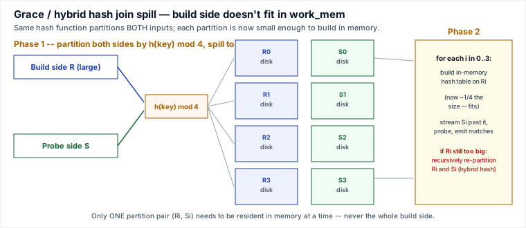
The reason this beats sorting the whole build side: sorting a relation that doesn’t fit in memory from scratch is O(n log n) over the entire dataset, while hash partitioning is a single linear pass to bucket the rows, after which each bucket is handled independently and cheaply. EXPLAIN (ANALYZE, BUFFERS) surfaces this directly in PostgreSQL as Batches: N on a Hash node — Batches: 1 means it fit in memory; anything higher means it spilled and partitioned.
Sargability: writing predicates an index can actually use
A predicate is sargable (“Search ARGument ABLE”) if the engine can push it straight into an index seek without first transforming every row’s value. The mechanism that breaks it: a B-tree index is ordered by the raw column value. The instant you wrap the column in a function, apply a leading wildcard, or force an implicit type conversion, the index’s ordering no longer corresponds to the thing you’re comparing — so the engine must transform every row to check the predicate, which is exactly what a sequential scan already does, except now with function-call overhead on top.
| Non-sargable (index unusable) | Sargable rewrite (index usable) | Why |
|---|---|---|
WHERE date(ts) = '2026-07-01' | WHERE ts >= '2026-07-01' AND ts < '2026-07-02' | date(ts) must be computed per row before comparing; the raw range on ts is a direct B-tree seek. (Alternative: build an expression index on date(ts) if the transform genuinely can’t be avoided.) |
WHERE email LIKE '%@gmail.com' | WHERE email LIKE 'john%' (for a prefix search), or a trigram/reverse-column index for suffix search | A leading % has no fixed prefix to seek to — the B-tree can’t narrow the range at all. A trailing wildcard ('john%') is sargable: the engine seeks to 'john' and scans forward until the prefix stops matching. |
WHERE phone = 5551234 (column is varchar) | WHERE phone = '5551234' | Comparing a text column to a numeric literal forces an implicit cast — often applied to the column side across every row — defeating the index; matching types keeps the comparison directly seekable. |
Three failure modes that don’t show up in a single EXPLAIN line
1. Cardinality error propagates up the tree
Every operator’s cost estimate is computed from its children’s row-count estimate, not the true row count. If a leaf scan under-estimates by 10× (stale statistics, a correlated predicate, an out-of-range value), that wrong number doesn’t stay local — it feeds directly into the parent join’s cost formula, which can flip the chosen join algorithm (a nested loop priced for 500 outer rows that actually receives 80,000 does 160× more probes than planned), and the join’s own now-wrong output estimate feeds the next join or sort above it. A single bad leaf estimate can silently determine the algorithm choice for an entire plan tree several levels up — which is why debugging a slow plan means walking EXPLAIN ANALYZE bottom-up to find the first node where estimated and actual rows diverge, not the top-level symptom.
2. Plan caching and parameter sniffing
A prepared statement (PREPARE p AS SELECT * FROM orders WHERE status = $1) can be planned once and reused. PostgreSQL builds a fresh “custom” plan (using the actual bound value’s real selectivity) for the first several executions, then may switch to a single cached “generic” plan built from an average/generic selectivity across all possible values. If status is skewed — 'shipped' is 90% of rows, 'refunded' is 0.1% — a generic plan tuned for the average case can be excellent for the rare value and disastrous for the common one, or vice versa, and it silently keeps running that way for every future call until re-planned. This “parameter sniffing” problem is why hot, skewed, parameterized queries sometimes need to be forced back to custom (per-call) planning rather than trusting the cache.
3. EXPLAIN ANALYZE executes the query
EXPLAIN alone only plans — it never touches data. EXPLAIN ANALYZE runs the query for real to measure actual timings and row counts, which means it also runs any side effect: a DELETE, UPDATE, or data-modifying CTE wrapped in EXPLAIN ANALYZE genuinely deletes or updates those rows. The safe habit:
BEGIN;
EXPLAIN ANALYZE DELETE FROM orders WHERE created_at < now() - interval '1 year';
ROLLBACK;
— real timings and row counts, zero committed changes.
Pitfalls a working engineer actually hits
- “The index exists but the planner won’t use it” is very often correct behavior above the selectivity crossover — check
EXPLAIN’s estimated rows before assuming the planner is wrong. - Forcing a plan (hints) before fixing the estimate. If the underlying cardinality estimate is wrong, forcing a join order or algorithm just masks today’s symptom; the same class of query misfires again the moment data shifts. Fix statistics/sargability first.
- A function-wrapped predicate silently disables an index with no error and no warning — it just runs a full scan and still returns the right answer, so it hides until the table grows large enough to hurt.
- A hash join reporting
Batches > 1means it spilled and partitioned — often fixable by raisingwork_mem, but only after confirming the build-side estimate itself is accurate (a bad estimate can make a hash join look like it “needs” to spill when the true build side would have fit). - Running
EXPLAIN ANALYZEon a DML statement in production without a transaction wrapper — it executes the mutation for real.
Judgment layer: how a senior engineer decides
- Index scan vs. seq scan: estimate (or check
EXPLAIN’s) selectivity. Below roughly a few percent — lower for narrow rows/cold cache, higher for wide rows/warm cache/correlated order — trust the index. Above it, a seq scan is very likely the right plan; don’t force an index hint without first checking whether the predicate is even sargable. - Which join algorithm: equality join, both sides large, unsorted → hash join (check the build side fits
work_mem). Either side already sorted on the key, or that order is needed downstream anyway → sort-merge. Any non-equality condition, or a small outer with a great index on the inner → nested loop; for a theta join, nested loop usually isn’t a planner choice so much as the only physically valid one, and the real fix is restructuring the predicate to add an equality component. - Trust a cached generic plan or not: if a parameterized predicate’s column is skewed (a handful of very common values among many rare ones — status flags, categories, boolean-like columns), a single generic plan is dangerous; either force custom re-planning for that query or keep it un-prepared. For uniform, low-skew columns (e.g. a UUID primary key lookup), a cached generic plan is safe and saves real replanning cost.
Takeaways
- Selectivity crosses over between index scan and seq scan because one cost is flat and the other grows linearly with matches — the exact crossover point shifts with row width, cache warmth, and index/heap correlation.
- Startup cost, not just total cost, decides the winner whenever a
LIMITis present — a “streaming” plan with a far higher full-run cost can beat a “blocking” plan with a lower one. - Hash and sort-merge joins only really support equality; any theta/inequality join condition forces nested loop, and grace/hybrid hashing lets a hash join scale past memory by partitioning both sides with the same hash function.
- Sargability, cardinality-error propagation, plan caching, and
EXPLAIN ANALYZE’s execution side effect are four ways a query gets slow (or dangerous) without a single glance at the plan tree revealing why.
Related pages
- How a Query Executes — Parse, Plan, Run & EXPLAIN — the iterator model and EXPLAIN basics this page builds on
- Join Algorithms — Nested Loop, Hash & Sort-Merge — companion page on join mechanics
- Indexing & Storage — Fanout Arithmetic, Optimizer Stats, Composite/Skip Scans & NULL/OR Pitfalls (Deep Dive) — index internals feeding sargability
- How Indexes Work — B+tree Internals — foundational B-tree structure this page assumes
- SQL Practice Patterns I — NULL Traps, COUNT Semantics, Sargability & the Missing-Group Pattern (Deep Dive) — sibling deep dive applying sargability to practice problems
Re-authored/Deepened for this guide.
🤖 Don't fully get this? Learn it with Claude
Stuck on Query Execution — Selectivity, the Cost Model, Join Algorithms, Spills & Sargability (Deep Dive)? Open Claude, copy a block below, and it'll teach you this exact concept — visually and interactively.
Build the mental picture, not memorization.
I just read a lesson on **Query Execution — Selectivity, the Cost Model, Join Algorithms, Spills & Sargability (Deep Dive)** (Databases) and want to truly understand it. Explain Query Execution — Selectivity, the Cost Model, Join Algorithms, Spills & Sargability (Deep Dive) from first principles using ONE vivid real-world analogy and a visual mental model — draw it as ASCII art or a clear step-by-step diagram — with a concrete example using real numbers. Then ask me one question to check I got the mental picture, and wait for my reply. If you're unsure or a claim isn't standard, say so and reason from first principles instead of guessing.
Socratic — adapts to where you're stuck.
Teach me **Query Execution — Selectivity, the Cost Model, Join Algorithms, Spills & Sargability (Deep Dive)** interactively. Ask me ONE guiding question at a time, wait for my answer, and adapt to my confusion — build the idea with me step by step instead of explaining it all at once. If you're unsure or a claim isn't standard, say so and reason from first principles instead of guessing.
Active recall exposes what you missed.
Quiz me on **Query Execution — Selectivity, the Cost Model, Join Algorithms, Spills & Sargability (Deep Dive)** with 5 questions, easy to tricky, ONE at a time. Tell me if each answer is right; at the end, explain clearly what I got wrong and why. If you're unsure or a claim isn't standard, say so and reason from first principles instead of guessing.
Intuition + hook + flashcards for long-term memory.
Help me remember **Query Execution — Selectivity, the Cost Model, Join Algorithms, Spills & Sargability (Deep Dive)** for the long term: give the one-sentence intuition, a memorable hook/mnemonic, a tiny worked example, and 3 active-recall flashcards (Q -> A). If you're unsure or a claim isn't standard, say so and reason from first principles instead of guessing.