Observability & SRE II — SLO Composition, Pipeline Failure Under Load, Latency Burn Rate & SRE Practice (Deep Dive)
An SLO is not a property of one service in isolation — it is a property of a request path, and the moment that path crosses a second service the arithmetic changes from addition to multiplication: every hard, synchronous dependency an incoming request must succeed through multiplies the whole chain’s availability down, never up, so a service built entirely from “three nines” dependencies cannot itself deliver three nines no matter how bug-free its own code is.
Why availability multiplies down a synchronous critical path
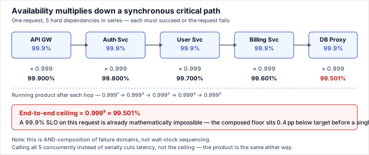
If a request must succeed through N independent hard dependencies in series — meaning the request fails if any one of them fails — the end-to-end success probability is the product of each link’s own availability, because success requires every link to succeed (a logical AND across independent failure domains). For 5 services each independently available 99.9% of the time:
| Hops composed | Expression | Running availability |
|---|---|---|
| 1 | 0.999¹ | 99.900% |
| 2 | 0.999² | 99.8001% |
| 3 | 0.999³ | 99.7003% |
| 4 | 0.999⁴ | 99.6006% |
| 5 | 0.999⁵ | 99.5010% |
0.999⁵ ≈ 0.995010, i.e. ≈ 99.5%. A team that sets its own SLO to 99.9% while sitting on top of five 99.9% dependencies has already lost 0.4 percentage points before writing a single line of code — the target was mathematically unreachable at design time, not missed through execution failure.
Whose budget burns? Cross-service error-budget attribution
Multiplication also answers a question every senior candidate gets asked: when a shared dependency degrades, which team’s error budget should the incident debit? Naively, the calling service’s SLI just fails and its own budget burns — but that silently blames the caller for a bug in someone else’s system.
Trace it with real numbers. Frontend F has a 99.9% SLO over a 30-day period (0.1% budget). One of its five hard dependencies, Auth Svc, has a bad deploy that drops its own availability from its normal 99.9% down to 99.0% for a full 24-hour day, then recovers.
| Quantity | Value |
|---|---|
| Excess unavailability at Auth Svc during the bad day | (1 − 0.990) − (1 − 0.999) = 1.0% − 0.1% = 0.9 percentage points |
| Fraction of F’s 30-day traffic that fell inside the bad day | 1 day / 30 days = 1/30 |
| Excess fraction of F’s monthly requests that failed solely because of Auth Svc | (1/30) × 0.9% = 0.03% |
| Share of F’s entire 30-day, 0.1% error budget consumed by that one dependency-day | 0.03% / 0.1% = 30% |
One 24-hour bad day at one dependency ate roughly a third of F’s entire monthly error budget — and if Auth Svc has four other consumers besides F, all five of them independently see the same 30% hit to their own budgets, from a single incident in a single team’s deploy.
Design implications
- Attribute burn per dependency, not just per SLI. Instrument a separate SLI per hard dependency (“success rate of my calls to Auth Svc”) alongside the end-to-end user-facing SLI. The user-facing SLI still fails — users do not care whose fault it is — but the policy decision (whose release freezes, who owns the postmortem) should route off the per-dependency SLI, debiting Auth Svc’s own budget and policy, not silently freezing every one of its five downstream consumers for a bug none of them can fix.
- A shared/critical dependency needs its own SLO and its own error-budget policy, sized for the fact that its failures fan out. If Auth Svc has five consumers, its own freeze threshold should arguably be stricter than any single consumer’s, since one bad day multiplies into five simultaneous incidents.
- Reduce the count of hard dependencies on the critical path — this is the only lever that changes the ceiling itself. Note precisely what “reduce sync depth” means: it is the count of mandatory, independent-failure-domain dependencies that multiplies, not whether they are invoked one-after-another or fanned out concurrently. Calling all five in parallel instead of serially cuts latency (bounded by the slowest call) but leaves the availability product exactly the same, because the request still needs all five to succeed. The only way to break a link out of the product is to make it non-mandatory: a cache that serves a slightly-stale answer when the dependency is down, a documented fallback/default, or making a feature best-effort so its failure degrades a response instead of erroring it.
- Demand tighter upstream SLOs, or fewer hard dependencies, before committing to a downstream target. If the business needs 99.9% and the design has five hard hops, either negotiate 99.98%+ from each dependency, or cut two of the five to optional/cached/fallback paths — the arithmetic is not negotiable, only the architecture is.
When the observability pipeline fails under the very incident it exists to diagnose
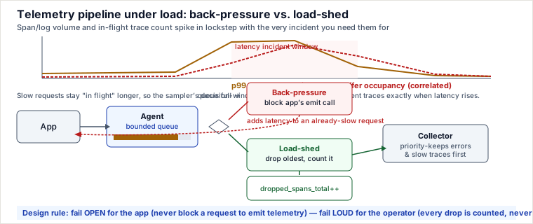
The pillars have a failure mode the emit-side cost model hides: telemetry volume does not stay constant during an incident — it spikes, exactly when you most need it, because clients retry failed calls (multiplying request count), error paths log more verbosely (stack traces, warn-level noise), and slow requests keep their trace spans “open” for longer. That last effect is the sharpest: tail-sampling holds every span of a trace in a buffer until the whole trace completes and a keep/drop decision is made, so the number of traces sitting in that decision-window buffer at any instant is roughly (arrival rate) × (average trace duration). When a latency incident stretches average trace duration, the buffer’s occupancy grows in lockstep with the incident itself — a self-correlated back-pressure that can exhaust collector memory at the exact moment engineers are staring at dashboards trying to find a slow trace.
Back-pressure vs. load-shed at agents and collectors
When an agent’s bounded emission queue fills — because the collector has slowed down or the emission rate has spiked — there are exactly two responses, and they trade off against each other in opposite directions:
- Back-pressure. The agent blocks the application’s emit call until the queue drains. This guarantees no telemetry is lost, but it injects extra latency directly into the request path of a service that is already in a latency incident — the cure makes the disease worse, and in the limit a synchronous, blocking telemetry client can turn a slow-response incident into a full outage.
- Load-shedding. The agent drops new data once the queue is full — typically oldest-first — and increments a
dropped_spans_total(ordropped_logs_total) counter so the drop itself is observable. The application keeps running at full speed; you lose some fidelity exactly when it is most valuable, but the user-facing incident does not get worse because of your instrumentation.
Production systems overwhelmingly choose load-shedding on the hot path, refined with priority sampling: rather than dropping data at random, shed healthy/fast traces first and always keep error traces and traces over a slow-latency threshold — precisely the traces useful for the incident. This is why tail sampling (a decision made only after the whole trace completes) can prioritize this way, and precisely why its buffer must hold every in-flight trace until that decision is made — the flexibility to keep “the interesting ones” is bought with the correlated-buffer-growth risk described above. Bound it: a hard per-collector trace cap, a short decision window (seconds, not tens of seconds), and shed-oldest-healthy-first so a crash loses only healthy, uninteresting traces, not the ones you needed. Metrics degrade differently again — a scrape that times out leaves a gap, not a wrong value, which is itself alertable (up == 0); that asymmetry is one reason metrics remain the primary alerting substrate even though logs and traces carry richer detail.
Because collector instances typically own a shard of trace IDs (consistent-hashed so all spans of one trace land on the same collector for the sampling decision), a collector crashing under this exact back-pressure loses every in-flight trace on its shard, with no replay — tail sampling is at-most-once trace capture, not a durable system of record. Treat it that way: keep the decision window short, do not try to replicate the buffer for durability, and lean on head-sampled coverage plus exemplar-pinned trace IDs (linking a slow metric bucket to at least one trace ID) as your fallback path to a trace when the tail sampler drops exactly the one you wanted.
Design implication: capacity headroom is a first-class SLO. Provision agent and collector capacity for worst-case incident telemetry volume — retries, verbose error logging, and elongated trace buffers — not average-case traffic, and monitor the observability pipeline itself (collector queue depth, drop-rate, WAL/replay lag) with its own alerts. If the pipe falls over during the incident it exists to explain, you are debugging blind at the exact moment stakes are highest.
Burn rate generalizes: it is not only about errors
Every burn-rate derivation on this topic so far has framed the “bad event” as an error. The formula generalizes to any SLI with a threshold: the bad event is simply “did this request violate the SLI’s target,” and:
burn_rate = (fraction of requests violating the SLI) / (1 - SLO_target)For a latency SLO of “95% of requests complete in under 300 ms” over a 30-day period, the bad event is “request took ≥ 300 ms,” the target is 95%, and the allowed budget is (1 − 0.95) = 5% of requests. Baseline “slow” fraction is normally ≈1% (burn rate 1/5 = 0.2, comfortably sustainable). At 10:00 a downstream timeout cascade pushes the slow-fraction to a sustained 80%, continuously, until a rollback lands at 11:00 (a full 60-minute incident, traced end to end exactly as the burn-rate-alerting page traces its error-rate example):
burn_rate = 80% / 5% = 16. Reusing the identical fast-burn tier from multi-window multi-burn-rate alerting (1h / 5m windows, multiplier 14.4), the corresponding threshold for this SLI is 14.4 × 5% = 72% of requests slow, not 1.44% of requests erroring — same machinery, different bad-event definition and a rescaled threshold because (1 − SLO) differs.
| Time | 5m window (short) | 1h window (long) | AND → PAGE? |
|---|---|---|---|
| 10:00 | rising | ≈1% (baseline) | no |
| 10:05 | 80% ≥ 72% ✓ | (55×1+5×80)/60 ≈ 7.58% ✗ | no (long not yet significant) |
| 10:54 | 80% ✓ | (6×1+54×80)/60 ≈ 72.1% ≥ 72% ✓ | PAGE |
| 11:00 | still 80% (rollback lands right at 11:00) | window 10:00–11:00, fully elevated → 80% ✓ | page holds |
| 11:05 | rollback took effect → ≈1% ✗ | window 10:05–11:05, 55 of 60 min elevated → (55×80+5×1)/60 ≈ 73.4% ✓ (still high) | RESET — short dropped, AND goes false even though the long window is still mathematically hot |
| 12:00 | ≈1% | window 11:00–12:00, entirely post-rollback → ≈1% ✗ | fully clear |
Detection time follows the same law as the error-rate case: t_detect ≈ (threshold_fraction × long_window) / actual_fraction = (72%×60)/80% = 54 min — which is exactly when the trace above pages. And the full 60-minute incident spends burn_rate × (window/period) = 16 × (60/43200) ≈ 2.22% of the entire 30-day latency budget. Nothing here is a new mechanism — it is the same MWMBR machinery from the burn-rate-alerting page, re-fed a latency-threshold SLI instead of an error-rate SLI, which is exactly the generalization a senior interviewer expects you to state unprompted.
SRE practice beyond the SLO math
Error budgets and burn rate are the quantitative core of SRE, but the operating model around them is what actually keeps a team sustainable and the postmortem data trustworthy.
- Blameless postmortems. The mechanism, not just the etiquette: a postmortem's only value is the information it extracts, and engineers who fear personal blame omit details, soften timelines, or delay reporting — starving the exact document meant to prevent recurrence. Blamelessness is therefore an instrumental choice for information quality, not a nicety: the template asks “what in the system allowed this” rather than “who did this,” the timeline is reconstructed from logs and multiple perspectives without naming an individual as the root cause, and action items target process, tooling, or architecture — things a future engineer can actually change.
- Toil budgets. Toil is manual, repetitive, automatable, tactical work that scales linearly with service growth and carries no enduring engineering value (ticket-driven restarts, manual failovers, copy-paste provisioning). Google’s canonical policy caps toil at ≤ 50% of an SRE’s time; when a team’s measured toil exceeds the cap, the team’s charter requires shifting engineering time into automation projects until it is back under the cap — a policy lever for engineering time, exactly parallel in structure to the error-budget freeze that governs reliability spend.
- On-call load and rotation health. Page volume, not just individual incidents, is itself a health metric: a rule-of-thumb ceiling of roughly two actionable pages per 12-hour on-call shift keeps response quality high, because an over-paged rotation degrades judgment and burns engineers out, which in turn degrades the very incident response the on-call system exists for. Track pages-per-week, off-hours (night/weekend) page rate, and time-to-acknowledge as trends; follow-the-sun rotations (handing the pager to a team in a different timezone at end-of-business) are a direct lever for cutting night pages without adding headcount.
- The error-budget policy’s escalation path, beyond the automatic freeze. The freeze itself — halt feature launches once the budget is exhausted — is the well-known mechanism; the part interviewers probe next is what happens when the business wants to override it. A mature policy names, in advance, who can grant a time-boxed exception (typically a director-level or cross-functional sign-off), requires the exception and its expiry to be logged alongside the incident record, and feeds a pattern of repeated overrides back into the next planning cycle as a signal that the team is systematically under-investing in reliability relative to feature velocity. Without a named escalation path, the freeze either gets silently ignored (and the policy loses all teeth) or blocks a genuinely critical launch with no legitimate way through.
Cardinality-bomb detection and triage playbook
Prevention (bounding label cardinality at the client) is necessary but not sufficient — you also need to localize a cardinality explosion while it is happening, to a specific metric name and the specific offending label, fast enough to stop an OOM before it takes the whole time-series database down.
- Alert on head-series growth rate, not just an absolute ceiling. Prometheus exposes total active series as the gauge
prometheus_tsdb_head_series. An absolute-ceiling alert (“page if > 5M series”) misses a bomb that is climbing fast but hasn’t yet crossed the line, and false-positives on a service that is legitimately, stably large. Instead alert on relative growth over a short window, e.g. a rule shaped like(prometheus_tsdb_head_series - prometheus_tsdb_head_series offset 1h) / prometheus_tsdb_head_series offset 1h > 0.2— a step-change after a deploy is exactly the signature of a new unbounded label going live, while a slow, steady rise from organic service growth stays under the rate threshold. - Find the fattest metric with
topkgrouped by name.topk(10, count by (__name__) ({__name__=~".+"}))counts active series per metric name across the whole namespace and returns the 10 largest. In a cardinality incident, one metric will dominate the list by one or two orders of magnitude — that is your suspect. - Find the offending label by counting its distinct values. Once you have a suspect metric, for each of its label names run
count(count by (<label>) (<metric_name>)): the inner query groups the metric’s series by that label’s value (one group per distinct value), and the outercount(…)counts how many distinct values exist. A normally low-cardinality label (environment, region, status class) should return single or double digits; a label secretly carrying a user ID, request ID, or raw URL path will return a number in the thousands-to-millions — that is the bomb. - Cross-check with Prometheus’s built-in endpoint.
/api/v1/status/tsdbexposes “top series count by metric name” and “top label value count by label name” directly from the TSDB’s internal stats, with zero PromQL evaluation cost — the fastest first move during an active incident when running expensive ad-hoc queries against an already-struggling TSDB is itself risky. - Mitigate at the source. Once the metric and label are identified: drop or relabel the label at scrape time (
metric_relabel_configswith anaction: labeldrop/replace), or fix the client library that is emitting it (the label almost always traces back to a recent deploy that started stamping a per-entity identifier onto a metric that was previously low-cardinality).
Pitfalls
- Treating fan-out (parallel calls) as if it reduces the availability ceiling. It reduces latency only. If the response still requires every one of N hard dependencies to succeed, the product is the same whether they are called serially or concurrently; only removing a dependency from the mandatory set changes the math.
- No per-dependency SLI, so one bad backend freezes ten unrelated teams. Without splitting “my own bugs” burn from “my upstream’s” burn, a shared dependency’s bad day trips release freezes across every consumer simultaneously, for a problem only one team can actually fix.
- Load-shedding without a drop counter. A collector that silently discards spans/logs when its queue is full turns “lossy under load” into “lying under load” — the drop itself must be a first-class, alertable metric, or nobody learns the observability data was incomplete during the very incident it was needed for.
- Applying error-rate MWMBR tiers to a latency SLI without checking the traffic floor. The identical low-traffic instability that plagues error-rate burn rate (a handful of requests making the ratio noisy) applies just as much to a fraction-over-threshold ratio — a latency SLI on a low-QPS endpoint needs the same minimum-sample guard.
- Blameful postmortems that look blameless on paper. Removing names from the document but still asking “who pushed the change” in the review meeting reintroduces the same chilling effect on honest reporting; blamelessness is a property of the process, not the template.
- A toil-budget cap nobody measures. A 50% ceiling is meaningless if toil hours are never actually logged — without measurement the policy is aspirational, and toil quietly consumes 80%+ of the team’s time while the dashboard says the cap is respected.
- Cardinality alerts on an absolute ceiling alone. A stable, legitimately large metric false-pages forever; a fast-growing new bomb that hasn’t yet crossed the line pages too late. Growth-rate, not just level, is the signal that matches the failure mode.
Selection and trade-offs
Back-pressure vs. load-shed on the telemetry hot path. Choose back-pressure only for telemetry you have already decided is more important than the request it is attached to — audit logs required for compliance, for example, where losing the record is a worse outcome than added latency. For ordinary observability data (metrics, traces, application logs) on a user-facing request path, load-shedding with a drop counter and priority sampling is almost always the right default: the alternative, back-pressure, converts an observability problem into an availability problem, which is the one failure mode a telemetry system must never cause. The exception that flips this: an internal batch/offline pipeline with no live user waiting, where blocking a producer briefly is genuinely free.
Reducing sync depth vs. accepting the composed ceiling. Cutting a hard dependency (cache-and-fallback, making a call optional, negotiating a tighter upstream SLO) is real engineering work with its own cost — cache staleness, added fallback-path complexity, or a harder negotiation with another team. It is worth paying when the composed ceiling sits below a target the business has already committed to externally (a contractual SLA, for instance) — there the math is not optional. It is not worth the churn when the composed ceiling already comfortably clears the target the business actually needs; matching architecture cost to the nines a user will notice, not the theoretical maximum, is the same judgment call that governs every reliability investment on this topic.
Takeaways
- Availability multiplies, never averages, down a synchronous critical path:
0.999⁵ ≈ 99.5%— a downstream SLO target can be mathematically unreachable before any code runs, and only removing a dependency from the mandatory set (not parallelizing it) changes the ceiling. - A shared dependency’s bad day should debit its own error budget via a per-dependency SLI, not silently freeze every consumer’s release — in the worked example, one 24-hour incident at one dependency consumed 30% of a single downstream team’s entire monthly budget.
- The observability pipeline is a system with its own failure modes that correlate with the incidents it diagnoses; the governing rule is fail open for the app, fail loud for the operator — and burn rate itself generalizes past error rate to any thresholded SLI via the same
bad_fraction / (1−SLO)formula. - SRE practice outside the SLO math — blameless postmortems, measured toil budgets, on-call load tracking, and a named error-budget escalation path — is what keeps the quantitative machinery trustworthy and the team sustainable enough to keep using it.
Recall question
A frontend with a 99.9% SLO calls five hard dependencies in series, each independently at 99.9%. One of them has a bad day and drops to 99.0% availability for 24 hours out of a 30-day period. Whose error budget should that incident debit, and why? (Answer: the failing dependency’s own error budget, via a per-dependency SLI tracked separately from the frontend’s end-to-end SLI — the frontend’s user-facing SLI still legitimately fails, since users experienced the outage, but the policy consequence, such as a release freeze, should route to the team that can actually fix the cause; otherwise every consumer of a shared dependency is punished simultaneously for a bug none of them own.)
Related pages
- SLIs, SLOs, SLAs & Error Budgets — the base definitions this page's SLO math builds on
- Burn-Rate Alerting — the MWMBR mechanism this page generalizes to latency SLIs
- Metrics, Logs & Traces — the Three Pillars — the pipeline whose failure mode under load this page covers
- Distributed Tracing & Exemplars — the tail-sampling and exemplar mechanics referenced here
- Tail Latency & Fan-out Amplification — Why p99 Is the Number — the fan-out/availability-composition math this page's opening section extends
Sources: Google SRE Book, ch. 4 “Service Level Objectives,” ch. 5 “Eliminating Toil,” and ch. 15 “Postmortem Culture”; Google SRE Workbook, ch. 2 “Implementing SLOs” and ch. 5 “Alerting on SLOs”; OpenTelemetry Collector documentation (tail sampling processor, queued-retry back-pressure); Prometheus documentation (TSDB head-series metrics, /api/v1/status/tsdb). Re-authored/Deepened for this guide.
🤖 Don't fully get this? Learn it with Claude
Stuck on Observability & SRE II — SLO Composition, Pipeline Failure Under Load, Latency Burn Rate & SRE Practice (Deep Dive)? Open Claude, copy a block below, and it'll teach you this exact concept — visually and interactively.
Build the mental picture, not memorization.
I just read a lesson on **Observability & SRE II — SLO Composition, Pipeline Failure Under Load, Latency Burn Rate & SRE Practice (Deep Dive)** (System Design) and want to truly understand it. Explain Observability & SRE II — SLO Composition, Pipeline Failure Under Load, Latency Burn Rate & SRE Practice (Deep Dive) from first principles using ONE vivid real-world analogy and a visual mental model — draw it as ASCII art or a clear step-by-step diagram — with a concrete example using real numbers. Then ask me one question to check I got the mental picture, and wait for my reply. If you're unsure or a claim isn't standard, say so and reason from first principles instead of guessing.
Socratic — adapts to where you're stuck.
Teach me **Observability & SRE II — SLO Composition, Pipeline Failure Under Load, Latency Burn Rate & SRE Practice (Deep Dive)** interactively. Ask me ONE guiding question at a time, wait for my answer, and adapt to my confusion — build the idea with me step by step instead of explaining it all at once. If you're unsure or a claim isn't standard, say so and reason from first principles instead of guessing.
Active recall exposes what you missed.
Quiz me on **Observability & SRE II — SLO Composition, Pipeline Failure Under Load, Latency Burn Rate & SRE Practice (Deep Dive)** with 5 questions, easy to tricky, ONE at a time. Tell me if each answer is right; at the end, explain clearly what I got wrong and why. If you're unsure or a claim isn't standard, say so and reason from first principles instead of guessing.
Intuition + hook + flashcards for long-term memory.
Help me remember **Observability & SRE II — SLO Composition, Pipeline Failure Under Load, Latency Burn Rate & SRE Practice (Deep Dive)** for the long term: give the one-sentence intuition, a memorable hook/mnemonic, a tiny worked example, and 3 active-recall flashcards (Q -> A). If you're unsure or a claim isn't standard, say so and reason from first principles instead of guessing.