Partitioning Methods
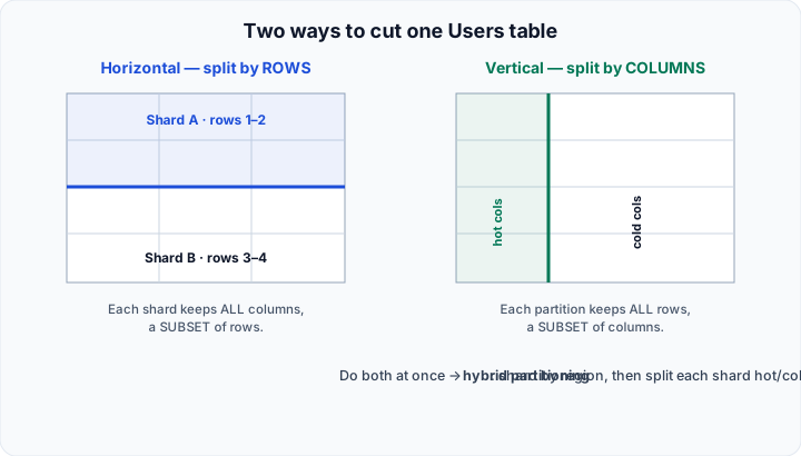
Partitioning means splitting one logical table across many physical stores so that no single machine has to hold — or serve — all of it. There are exactly two axes you can cut along, and every named scheme is a combination of the two:
- Horizontal partitioning (sharding) cuts along rows. Every shard has the full set of columns but only a subset of the rows — e.g. Americas users here, Europe users there.
- Vertical partitioning cuts along columns. Every partition has the full set of rows but only a subset of the columns — e.g. the small, hot profile fields in one store and the large, cold blobs in another.
A single table can be cut both ways at once; that combination is called hybrid partitioning. Keep the two axes straight and the rest of this lesson — including the trade-offs — falls out cleanly.
Horizontal partitioning (sharding)
You pick a partition key — say, the user's home region — and route each row to a shard based on that key. A login for a US user touches only the Americas shard; the other shards never wake up for that request. This buys three things: each node holds less data, queries scan less, and writes that used to contend for one machine's CPU, locks, and disk are now spread across N independent machines, which raises the write ceiling.
The whole scheme lives or dies by the key. If the key's values aren't evenly distributed across shards, you get skew: some shards run hot while others idle, and your slowest shard — not your average shard — defines your tail latency and your capacity ceiling. Partitioning users by geography quietly assumes regions are evenly populated. They are not.
Worked example: what skew actually costs you
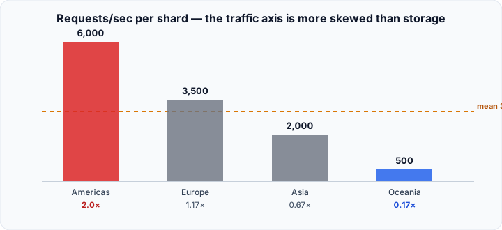
Take 100M users across 4 region shards, serving 12,000 requests/sec in total. If the load were perfectly even, every shard would hold the mean of 25M rows and serve the mean of 3,000 QPS. Real geography looks more like this:
| Shard | Region | Rows | Rows vs mean | QPS | QPS vs mean |
|---|---|---|---|---|---|
| 0 | Americas | 45M | 1.8× | 6,000 | 2.0× |
| 1 | Europe | 30M | 1.2× | 3,500 | 1.17× |
| 2 | Asia | 20M | 0.8× | 2,000 | 0.67× |
| 3 | Oceania | 5M | 0.2× | 500 | 0.17× |
Note that the skew is worse on the traffic axis than on the storage axis, because active users cluster even more tightly than raw accounts. Shard 0 (Americas) carries 1.8× the mean on rows but 2.0× on QPS — it is your bottleneck, and you must provision every shard's hardware for it or watch it fall over. Shard 3 (Oceania) sits at one-fifth of the mean on rows and only about one-sixth (0.17×) on QPS — nearly idle capacity you are paying for. The rows-to-QPS mismatch is the whole point: a key that balances storage can still leave traffic lopsided.
So Americas is 2× hot — what do you actually do? Three exits, in escalating cost: (1) split the hot range — Americas becomes Americas-East/Americas-West, two shards each at roughly 1.0× the mean (this works because range boundaries are editable; it is exactly what dynamic partitioning automates — see Rebalancing Strategies); (2) go hybrid — keep geo routing for residency, but consistent-hash user_ids within each region so a region's load spreads over k nodes (see Data Sharding Techniques); (3) re-key entirely to hash(user_id) — perfect balance, but you forfeit region locality and pay a full one-time migration. Choose (1) when the skew is between coarse ranges, (2) when residency law pins the outer key, and (3) only when the locality was never actually used.
Choosing the key: range vs. hash
There are two ways to map a key to a shard, and picking between them is the first real judgment call in sharding:
- Range partitioning keeps ordered keys together (region, or user_id 0–25M on shard 0, 25M–50M on shard 1, and so on). You keep locality: range scans and “next 50 rows” queries hit one shard. The price is skew and hotspots — a popular range (Americas, or the newest user_ids everyone is writing) overloads one shard, exactly as the table above shows.
- Hash partitioning routes on
hash(key) mod N. You get near-perfect balance because the hash scatters even a lopsided key distribution evenly. The price is lost locality: adjacent keys land on different shards, so range scans must fan out to every shard, and you can no longer answer “the next N users” from one place.
So the trade is balance (hash) vs. locality (range). Reach for range when your dominant query is a scan over ordered keys; reach for hash when your dominant query is a point lookup and even load matters more than ordering. One footgun with plain mod N: changing N reshuffles almost every key. The fix — consistent hashing — is covered in the next lesson, Data Sharding Techniques.
See it: hash vs. consistent hashing on the ring
Hash sharding with plain hash(key) mod N looks fine — until you add or remove a node and almost every key remaps. The debugger below runs 120 keys through modulo, consistent hashing, and consistent hashing + virtual nodes. Step the node crash scenario and predict how many keys move — that number is the interview answer.
Vertical partitioning
Instead of cutting rows, you cut columns: pull the small, hot, frequently-read fields into one store and leave the large, cold, rarely-read ones in another. It pays off when a row mixes both.
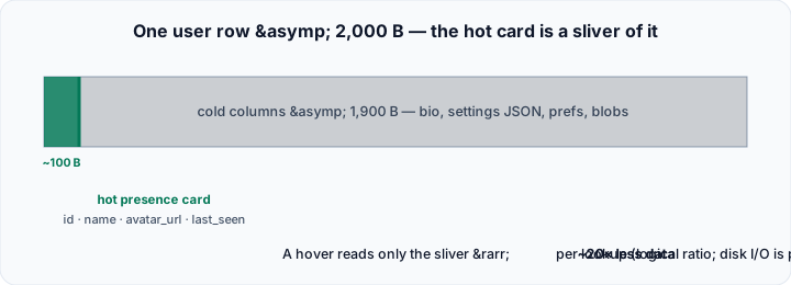
Take a user row that is roughly 2 KB — most of that is a bio, JSON settings, denormalized blobs, and preferences that a profile-hover almost never needs. The hot “presence card” a hover does need is just id, name, avatar_url, and last_seen. Budget it honestly: id 8 B + name ~20 B + avatar_url ~60 B (a URL alone is usually 60–100 B) + last_seen 8 B ≈ ~100 B — not the ~40 B an over-optimistic estimate might suggest. Splitting the hot card into its own narrow table means a hover reads ~100 B instead of ~2 KB: about 20× less data per lookup.
Read that 20× as a logical row-size ratio, not a literal disk-I/O figure. Real reads are page/block-granular, so the exact I/O saving depends on how many rows share a page and on caching. But because vertical partitioning physically separates the hot columns, a narrow hot table packs many more presence cards per page — so the direction is right and the win is real, just not a clean 20× at the block layer.
Hybrid partitioning
Real large systems combine both axes. Shard the users table horizontally by region, then vertically split each shard into a hot presence store and a cold profile store. A US profile-hover is then a point read of ~100 B from a single shard's hot store — small on both axes at once. That compounding is the appeal, but so does the operational cost: you now maintain two split strategies, and a query that needs cold columns for a range of users pays both a cross-shard fan-out and a hot-to-cold join.
The pitfalls any split introduces
Both cuts break the one thing a single table gave you for free — the ability to answer a query from one place:
- Cross-shard joins. Once rows for a join live on different shards, the database can't join them locally; you fan out, ship partial results, and stitch them in the app or a coordinator. Latency tracks your slowest shard.
- Distributed transactions. A write touching two shards (or a hot and a cold vertical partition) can no longer rely on a single node's ACID guarantee. You reach for two-phase commit or sagas — both slower and more failure-prone than a local transaction.
- Rebalancing. When a shard gets hot, moving keys elsewhere is real data movement under live traffic — the problem consistent hashing is designed to shrink.
When to use it — and when not
Reach for horizontal partitioning when a single table's data volume or write throughput genuinely exceeds what one well-indexed node (plus read replicas) can serve. Then pick the key by your dominant access pattern: range for scan-heavy, ordered workloads (accept the hotspot risk); hash for point-lookup workloads where even load matters more (accept the loss of range locality).
Reach for vertical partitioning when a single row mixes a small, hot, frequently-read column group with large, cold, rarely-read columns — the presence-card-vs-blob shape above.
When not to:
- Don't shard prematurely. A single well-indexed node with read replicas and caching handles far more than people expect. Sharding is a one-way door that buys scale by spending simplicity — cross-shard joins, distributed transactions, and rebalancing all arrive together. Exhaust the single-node path first.
- Don't over-eagerly vertical-split. Every column group you can't answer from one partition turns a single-row read into a multi-partition read plus a join. Split only when the hot/cold access divide is real and lopsided; splitting columns that are almost always read together just manufactures joins for no I/O win.
- Don't cut along an axis your queries don't follow. A key that balances storage but not traffic (or a vertical split that severs columns your hottest query needs together) makes things worse, not better — always cut along the access pattern.
Sources
Adapted and expanded from the “Partitioning Methods” lesson in this System Design track, with the worked skew example, honest byte budget, and range-vs-hash / when-not-to trade-off analysis added for depth. For a rigorous treatment of partitioning, skew and hotspots, and rebalancing, see Martin Kleppmann, Designing Data-Intensive Applications (O'Reilly, 2017), Chapter 6, “Partitioning.” Consistent hashing is covered in the next lesson, Data Sharding Techniques.
🤖 Don't fully get this? Learn it with Claude
Stuck on Partitioning Methods? Open Claude, copy a block below, and it'll teach you this exact concept — visually and interactively.
Build the mental picture, not memorization.
I just read a lesson on **Partitioning Methods** (System Design) and want to truly understand it. Explain Partitioning Methods from first principles using ONE vivid real-world analogy and a visual mental model — draw it as ASCII art or a clear step-by-step diagram — with a concrete example using real numbers. Then ask me one question to check I got the mental picture, and wait for my reply. If you're unsure or a claim isn't standard, say so and reason from first principles instead of guessing.
Socratic — adapts to where you're stuck.
Teach me **Partitioning Methods** interactively. Ask me ONE guiding question at a time, wait for my answer, and adapt to my confusion — build the idea with me step by step instead of explaining it all at once. If you're unsure or a claim isn't standard, say so and reason from first principles instead of guessing.
Active recall exposes what you missed.
Quiz me on **Partitioning Methods** with 5 questions, easy to tricky, ONE at a time. Tell me if each answer is right; at the end, explain clearly what I got wrong and why. If you're unsure or a claim isn't standard, say so and reason from first principles instead of guessing.
Intuition + hook + flashcards for long-term memory.
Help me remember **Partitioning Methods** for the long term: give the one-sentence intuition, a memorable hook/mnemonic, a tiny worked example, and 3 active-recall flashcards (Q -> A). If you're unsure or a claim isn't standard, say so and reason from first principles instead of guessing.