Design a Metrics / Log Pipeline
Design a Metrics / Log Pipeline
Every candidate can draw the four boxes: "agents send metrics, we store them in a database, dashboards query it, done." That answer survives about ten seconds. The instant the interviewer says "you have 10,000 hosts each emitting 1,000 metrics every 10 seconds" the naive design is already on fire — that's one million data points per second, forever, and you just proposed writing each one as a row to a SQL table and running SELECT ... GROUP BY on read. This lab is about the two ideas that actually make a monitoring system (Datadog / Prometheus / a centralized log-analytics platform) work at that scale and that almost nobody names unprompted: pre-aggregation on the write path (you roll raw points into time-window summaries as they arrive, you don't store-then-aggregate) and downsampling into retention tiers (recent data is high-resolution, old data is coarse). Miss those two and no amount of sharding saves you. The third thing that quietly kills these systems — cardinality — isn't a scaling knob at all; it's a data-model landmine one careless engineer steps on. We derive all three from first principles, with the arithmetic shown.
Movement 1 — The Trap: "just write every point to a database and query it"
Here is the design that feels complete and is a disaster. One row per metric point in a relational table:
-- THE TRAP
CREATE TABLE metrics (
  metric_name TEXT, host TEXT, tags JSONB,
  ts TIMESTAMPTZ, value DOUBLE PRECISION
);
-- write path: one INSERT per incoming point
-- read path: SELECT avg(value) FROM metrics
--            WHERE metric_name='cpu.util' AND ts > now() - '24h'
--            GROUP BY time_bucket('1m', ts);
Now feed it the stated load. 10,000 hosts × 1,000 metrics = 10 million active time series; each emits one point every 10s, so:
points/sec = 10,000,000 series × (1 point / 10s) = 1,000,000 points/sec
points/day = 1,000,000 × 86,400 = 86,400,000,000  ≈ 86.4 BILLION rows/day
Write side melts first. No single Postgres/MySQL primary ingests ~1M row-inserts/sec sustained — you're an order of magnitude past what a B-tree-index-per-write engine does before write amplification and index bloat stall it. Even batched, you're appending 86.4B rows/day; the secondary indexes alone (you'd need one on (metric_name, ts)) rewrite constantly. Within hours the table is tens of TB and every INSERT is fighting a multi-hundred-GB index.
Read side is worse. A dashboard asking "p99 CPU across the fleet, last 24h" must scan every raw point in that window: 10,000 hosts × 8,640 points/host/day = 86.4 million rows scanned for one panel, sorted to compute a percentile, on every refresh. A dashboard has 30 panels; ten engineers have it open. You are now scanning billions of rows per second on read. The database doesn't slow down — it falls over.
And the silent killer: someone adds a tag request_id (or user_email, or a raw url) to a metric. Each distinct tag value is a new time series. One unbounded tag turns 1 series into millions (Movement 5 traces the exact blast radius). The table schema happily accepts it, and your ingester runs out of memory two hours later. The trap isn't one mistake; it's that the obvious design has no defense against volume or cardinality. See Metrics, Logs & Traces — the Three Pillars for why metrics specifically demand a different engine than logs.
Movement 2 — Scope it like a senior (ask before you draw)
Do not draw boxes yet. Each of these answers moves the design materially:
- Metrics, logs, or traces? They are not one system. Metrics are numeric, regular, massively compressible, and pre-aggregatable (this lab's focus). Logs are high-entropy text you can't pre-aggregate the same way (you index/search them — ELK/Loki shape). Traces are causal spans, usually sampled. Conflating them is the most common scoping miss. Pin which one dominates.
- Push or pull ingestion? Do agents push to a gateway (StatsD/Datadog-agent style) or does the system pull/scrape targets (Prometheus style)? This decides service discovery, backpressure ownership, and how "a host went dark" is detected. (Trade-off table, Movement 6.)
- Retention & rollups? How long must data live, and at what resolution over time? "10s resolution for 13 months" vs "10s for a week, 1-min for a month, 1-hr for a year" differ by ~15× in storage (computed in Movement 4). This is the single biggest cost lever.
- Query latency SLA? Interactive dashboards want p99 < ~1s on recent data; ad-hoc historical analytics can tolerate seconds. This decides how aggressively you must pre-aggregate vs compute on read.
- Cardinality expectations? What tags are allowed, and are any high-cardinality (user_id, request_id, url)? Get a hard "no unbounded tags" contract or design an enforcement point — see The Cost of Observability — Cardinality.
- Exact or approximate? Must a distinct-count / percentile be exact, or is a bounded-error estimate fine? "Exact p99 across a fleet" means storing or shuffling every sample; "approximate p99 within ~1%" unlocks mergeable sketches (t-digest) and is almost always the right call for monitoring. This one answer reshapes the whole aggregation layer.
Assume for this lab: metrics (numeric time series), push ingestion via agents; tiered retention (raw 10s / 1-min / 1-hr); interactive dashboards need p99 < 1s on recent windows; tags are bounded by contract but the system must defend against violations; percentiles and distinct-counts may be approximate (bounded error). 10K hosts × 1K metrics × 1 point/10s. This is a Prometheus/Datadog-scale internal platform, not multi-tenant SaaS.
Movement 3 — Reason to the design (derive it, don't recite it)
Attempt 1 — store raw, aggregate on read (the Trap). Fails on both write throughput (~1M inserts/s) and read fan-out (86.4M rows/panel). The lesson: at this volume you cannot afford to touch every raw point at query time. So push the aggregation earlier.
Attempt 2 — pre-aggregate on the write path. As points stream in, group them by (series, time-window) and compute the summary once: for a 1-minute window of a series you keep count, sum, min, max, last instead of the 6 raw points. Now "average CPU per minute" is a read of one pre-computed row per minute, not a scan-and-group of six. The insight generalizes: the read cost of an aggregate should be paid once, at write time, not re-paid on every query. This is why a metrics system is fundamentally a stream-processing problem, not a database-query problem — see Batch vs Stream Processing and Windowing & Watermarking in Streaming Systems.
But percentiles don't sum. You can add two windows' counts and sums to merge them, but you cannot compute p99-of-the-hour by averaging twelve 5-minute p99s — percentiles aren't distributive. Two escapes: (a) store every sample so you can re-percentile exactly (back to the volume problem), or (b) store a mergeable sketch per window — a t-digest for percentiles, HyperLogLog for distinct-counts. A t-digest is a few KB that answers "what's p99?" within ~1% error, and crucially two t-digests merge into one. So "p99 across the fleet for the hour" = merge N small sketches, not scan N million points. This is the same probabilistic-structure trade you'd make with a Bloom filter: give up exactness to collapse space and make results composable. (Full follow-up in Movement 7.)
Attempt 3 — decouple ingest from aggregation with a buffer. If the aggregator does synchronous work per point, a slow aggregator backs pressure straight onto the agents (or drops data). Put a Kafka log between ingest and aggregation, partitioned by hash(series-id) so all points of a series land on one partition (ordered, and one aggregator owns each series' windows). The log is the shock absorber: a GC pause or a redeploy of the aggregator just grows consumer lag, which the buffer holds until the consumer catches up — no data loss, no agent-side backpressure. See Kafka Partitions — Parallelism & Ordering and Back-Pressure Mechanisms — block, drop, or shed.
Attempt 4 — downsample old data into tiers. Nobody debugging a 6-month-old incident needs 10-second resolution — they need the shape. So run a rollup job that turns raw into progressively coarser resolutions and expires the fine ones: raw 10s kept 7 days, 1-min kept 30 days, 1-hr kept 13 months. This is ~15× less storage than keeping everything raw (Movement 4), and it makes historical queries fast because they read the already-coarse tier. This is the whole game: pre-aggregate on write, downsample over time.
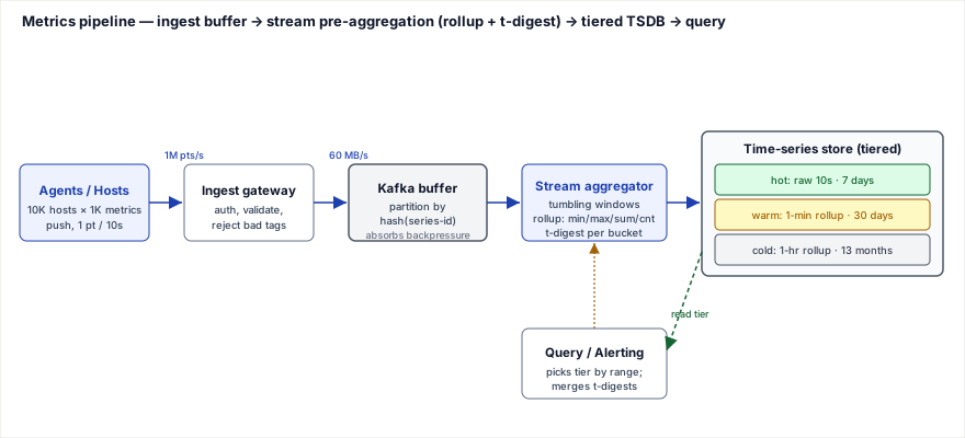
That chain — agents → ingest gateway → Kafka buffer (partition by series) → stream aggregator (windowed rollup + t-digest) → tiered TSDB → query layer — is the design. The rest is arithmetic and defending the choices.
Movement 4 — Build it: the design worksheet
This is the artifact you'd produce on the whiteboard. Numbers are traced, not asserted — recompute them before an interview.
1. Requirements
Functional: ingest numeric points (series-id, tags, ts, value) via push; pre-aggregate into time-window rollups; store at tiered resolution; query by metric + tag filter + time range + aggregation (avg/sum/rate/p99); fire alerting rules on the aggregated stream.
Non-functional: sustain ~1M points/s ingest with headroom; no data loss on aggregator restart (durable buffer); dashboard reads p99 < 1s on recent tiers; storage bounded by retention policy; must survive a bad high-cardinality tag without full outage (degrade, don't die).
2. Back-of-envelope estimation (arithmetic shown)
- Active series: 10,000 hosts × 1,000 metrics/host = 10,000,000 series.
- Ingest rate: each series = 1 point / 10s = 0.1 pt/s → 10M × 0.1 = 1,000,000 points/s. ×86,400 s/day = 86.4 billion points/day.
- Ingest bandwidth: wire point (protobuf remote-write: interned series ref + 8B ts + 8B float + framing) ≈ 60 bytes. 1M/s × 60 B = 60 MB/s ≈ 480 Mbps uncompressed; Snappy on the transport (~3×) brings the network to ~20 MB/s. Trivial bandwidth — the cost is storage and CPU, not the pipe.
- Stored bytes/point: logically 16 B (8B ts + 8B float64). Time-series compression — delta-of-delta on timestamps + XOR on floats (Gorilla-style) — observed ~1.3 B/point in production; use 2 B/point conservatively.
- Raw-resolution storage: 86.4B pts/day × 2 B = 172.8 GB/day ≈ 173 GB/day compressed at full 10s resolution.
- If you kept everything raw for 13 months (395 days): 172.8 GB × 395 ≈ 68 TB. This is the number tiering must beat.
Tiered retention (the key saving), computed:
Tier 0  raw 10s, keep 7 days
        86.4B pts/day × 2 B = 172.8 GB/day × 7   =  1.21 TB

Tier 1  1-min rollup, keep 30 days
        pts/day = 10M series × 1,440 min = 14.4B/day   (6× fewer than raw)
        rolled point holds ~5 aggregates ≈ 6 B compressed
        14.4B × 6 B = 86.4 GB/day × 30            =  2.59 TB

Tier 2  1-hr rollup, keep 13 months (395 days)
        pts/day = 10M series × 24 = 240M/day        (360× fewer than raw)
        240M × 6 B = 1.44 GB/day × 395            =  0.57 TB
        --------------------------------------------------------
        TOTAL tiered 13-month footprint            ≈  4.37 TB
68 TB ÷ 4.37 TB ≈ 15× less storage for the same 13-month retention — and historical queries hit the pre-coarsened tier, so they're fast too. That one design decision (downsampling) is worth more than any sharding cleverness.
- Kafka buffer sizing: at 60 MB/s, a 6-hour safety retention = 21,600 s × 60 MB/s ≈ 1.3 TB of buffered log — that's how long the aggregator can be down/lagging before data expires. Cheap insurance.
3. API sketch
// WRITE (push, batched)
POST /v1/ingest
     body: [ { series: "cpu.util", tags:{host,dc,role}, ts, value }, ... ]
     -> 202 Accepted            // buffered to Kafka, aggregated async
     -> 429 CARDINALITY_LIMIT   // series budget for this tag-set exceeded

// READ
GET /v1/query
     ?metric=cpu.util
     &filter=dc="us-east",role="web"
     &from=...&to=...
     &step=1m
     &agg=p99          // avg|sum|rate|min|max|p50|p99|count_distinct
     -> 200 { series:[ { tags, points:[[ts,value],...] } ] }
     // query planner picks the tier whose resolution ≤ requested step
4. Data model & partitioning
- Series identity:
series-id = hash(metric_name + sorted(tags)), interned once in an inverted index (tag=value → set of series-ids) so filters resolve to series sets without scanning data. - Partition key =
hash(series-id). All points of a series go to one Kafka partition and one aggregator instance — so a series' window state is owned by exactly one consumer (no cross-node coordination to close a window), and load spreads evenly across 10M series. Partitioning by time instead would create a hot partition (all writes hit "now"); partitioning by series avoids that. See Data Sharding Techniques. - Storage engine = LSM-tree / columnar TSDB (append-optimized), not a B-tree relational store: writes are append-only, sorted by (series, ts), and columnar layout lets the Gorilla compression above kick in. See Storage Engines — How B-tree & LSM-tree Work.
- Hot vs cold: recent (last few hours, raw tier) stays in an in-memory head block for sub-second reads; sealed older blocks flush to disk/object storage. Query planner routes by time range × requested step to the coarsest tier that still satisfies resolution.
5. High-level diagram
Write path (blue): agents push → gateway validates & rejects bad tags → Kafka buffers, partitioned by series → stream aggregator computes windowed rollups + a t-digest per (series, window) → tiered TSDB. Read path (green): query/alerting layer picks the tier by range and merges t-digests rather than scanning raw points.
6. Rubric — what a strong answer hits
- Computes the ingest rate (1M pts/s) and daily volume (86.4B) out loud before proposing storage — and immediately rejects "row per point in SQL" on that basis.
- Names pre-aggregation on write and downsampling into retention tiers as the two core ideas, and quantifies the tiering saving (~15×).
- Recognizes percentiles aren't distributive and reaches for a mergeable sketch (t-digest / HLL) instead of storing every sample.
- Puts a durable buffer (Kafka) between ingest and aggregation and explains it as backpressure absorption, partitioned by series for ordered per-series windowing.
- Treats cardinality as a first-class hazard with an enforcement point, not an afterthought.
- Picks push-vs-pull deliberately and can defend the storage engine (LSM/columnar TSDB, not B-tree relational).
Movement 5 — Break it: three traced failures
1. Cardinality explosion — the landmine, traced. Total series = the product of each tag's distinct-value count, because every unique tag combination is its own series. An engineer instruments a metric http_requests_total with tags customer_id, endpoint, status. Looks harmless. But:
series = |customer_id| × |endpoint| × |status|
       = 200,000       × 500        × 5
       = 500,000,000 series   from ONE metric
That's 50× the entire rest of the fleet (10M) from a single careless tag. The aggregator keeps active-window state per series in memory; at even ~3 KB of head + index per series, 500M series = ~1.5 TB of RAM for one metric → the ingester OOMs and takes down ingestion for everyone. The fix is an enforcement point, not more RAM: the ingest gateway tracks per-metric series budgets and returns 429 CARDINALITY_LIMIT (and drops/aggregates-away the offending tag) once a metric blows past its allotted series count — contain the blast to the bad metric. Distinct-value counts themselves are tracked cheaply with HyperLogLog, not exact sets. See The Cost of Observability — Cardinality.
2. Ingestion backpressure / Kafka lag, traced. The aggregator hits a stop-the-world GC pause, or you redeploy it. It stops consuming for 90 seconds. Producers keep pushing at 1M pts/s, so consumer lag grows at 1M points/s × 90s = 90M buffered points. Because Kafka is a durable log (not an in-memory queue), that's fine — it's ~90M × 60 B ≈ 5.4 GB of lag sitting safely in the 1.3 TB buffer, and the consumer drains it on restart. Without the buffer (agents pushing straight to the aggregator), those 90s of points have nowhere to go: the aggregator's socket buffers fill, agents either block (backpressure climbs the whole chain to the monitored apps — you can't let monitoring stall production) or drop points silently (you lose visibility exactly when something is wrong). The buffer converts "cascading backpressure or data loss" into "bounded, recoverable lag." The bound to watch: if the aggregator is down longer than the 6-hour retention, the oldest lag expires and is lost — so alert on consumer-lag-time approaching retention. See Kafka — Delivery Semantics & Producer Back-Pressure.
3. Query fan-out over unrolled raw data, traced. "p99 latency across all 10K hosts, last 24h" against the raw tier: 10,000 hosts × 8,640 points/host/day = 86.4 million points to fetch, merge, and sort for one panel — per refresh. With pre-aggregation, the aggregator already wrote one t-digest per (metric, 1-min window); 24h = 1,440 windows, so the query fetches and merges 1,440 small sketches and reads the answer off the merged digest. That's 86.4M ÷ 1,440 ≈ 60,000× less work, and it's why the p99 < 1s SLA is even possible. The raw tier exists for "zoom into this one series for 5 minutes during an incident," not for fleet-wide aggregate queries — those must hit pre-aggregated sketches.
Movement 6 — Optimise, with trade-offs vs named alternatives
| Decision | Option A | Option B | Pick when |
|---|---|---|---|
| Ingestion model | Pull / scrape (Prometheus) | Push (StatsD / Datadog agent) | Pull buys you free liveness detection (a target that won't scrape is down) and central control of scrape rate, but needs service discovery and struggles with short-lived jobs and NAT/firewalls. Push handles ephemeral jobs, serverless, and cross-network agents, and moves rate control to the client — but you lose "silence = down" and must defend the gateway against floods. Push for heterogeneous/ephemeral fleets; pull for a stable, discoverable service mesh. |
| When to aggregate | Aggregate-on-read (store raw, GROUP BY at query) | Pre-aggregate-on-write (windowed rollup in the stream) | Aggregate-on-read keeps full fidelity and supports arbitrary ad-hoc queries, but re-pays the scan cost on every query — fine at low volume, fatal at 86.4B pts/day. Pre-aggregate-on-write pays once and makes dashboards O(windows) not O(points), at the cost of committing to your aggregation functions up front (you can't retroactively compute an aggregate you didn't roll up). Pre-aggregate for known dashboard/alert queries; keep a short raw tier for the ad-hoc/incident case. |
| Percentiles & distinct-counts | Exact (store/shuffle every sample) | Probabilistic sketch (t-digest for percentiles, HyperLogLog for distinct) | Exact is required for billing or compliance where a number must be defensible to the cent; it costs O(all samples) storage and non-mergeable computation. Sketches give bounded error (t-digest ~1% on tail quantiles; HLL ~2% on cardinality) in a few KB, and — the property that matters — they merge associatively, so fleet-wide p99 = merge of per-window sketches. Use sketches for monitoring; exact only when the number is contractual. |
| Storage engine | B-tree relational (Postgres, sharded) | Columnar / LSM TSDB (Gorilla-style) | B-tree relational gives you joins, ad-hoc SQL, and strong transactions — none of which a metric point needs — while its per-write index maintenance is exactly what dies at 1M inserts/s. A columnar/LSM TSDB is append-optimized, sorts by (series, ts), and unlocks delta-of-delta + XOR compression (~2 B/point vs ~16 B raw). Always the TSDB here; reach for relational only if metrics must join transactionally against business entities (rare). |
| Rollup execution | Streaming rollup (continuous, in the aggregator) | Batch rollup (periodic job over raw) | Streaming keeps rollups fresh (alerts fire on near-real-time aggregates) but the windowing/late-data logic lives in the hot path. Batch is simpler and reprocessable (recompute a tier if the logic was wrong) but adds latency and re-reads raw. Stream the recent tiers for alerting freshness; batch the deep downsampling (1-hr tier) where latency doesn't matter. See Stateful Stream Processing — Checkpoints, Restart & TTL. |
Movement 7 — Defend under drilling
Q1 — "Why not just throw the raw points in a big data lake and query with Spark?"
Because the dominant workload is interactive dashboards and alerting with a sub-second SLA, and a lake/Spark scan of 86.4M points per panel is seconds-to-minutes, not sub-second. A lake is a fine cold archive or ad-hoc analytics backstop, but the serving path must be a purpose-built TSDB with pre-aggregated tiers. Different tool for a different read pattern — I'd keep both: TSDB for serving, object storage for cheap long-term raw archive if compliance needs it.
Q2 — "How do you compute p99 latency across the whole fleet without storing every sample?"
The aggregator maintains a t-digest per (metric, time-window) instead of the raw samples. A t-digest is a compressed, variable-resolution summary of a distribution — it keeps fine-grained centroids in the tails (where p99/p999 live) and coarse ones in the middle, so it answers extreme quantiles accurately in a few KB regardless of how many samples fed it. The property that makes it work at fleet scale: t-digests merge — combining the digests of two windows (or two hosts) yields a digest that answers as if you'd pooled all their samples. So fleet-wide p99 for the hour = merge the ~600 per-window/per-host digests and read p99 off the result — no sample ever leaves the host in raw form, and the answer is within ~1%. (Same reasoning: HyperLogLog for "how many distinct users," count-min for heavy-hitters — mergeable, sublinear, bounded-error. The exact-vs-approximate scoping question, Movement 2, is what licenses this.) It's the same space-for-exactness trade as a Bloom filter.
Q3 — "A whole dashboard team says their p99 graph looks wrong after a deploy. What's your first suspicion?"
Averaged percentiles. If some layer is computing p99-of-p99s (e.g., a rollup that stored per-minute p99 as a plain number and then the query averages those), that's mathematically meaningless and typically under-reports the real tail. The fix is that the rollup must store the mergeable t-digest, not a scalar p99, so the query re-derives the true quantile from merged digests. This is the single most common percentile bug in real monitoring systems.
Q4 — "Late-arriving data: an agent's network blipped and points for 10:00 arrive at 10:07, after you closed the 10:00 window. What happens?"
This is the streaming watermark problem. Options: (a) hold windows open for a grace period (watermark lag) before sealing — costs memory and delays the rollup; (b) seal on time and route late points to a correction path that re-opens/patches the affected window in the TSDB; (c) drop them past a bound and accept slight undercount. For monitoring I'd use a small grace period (say 1–2 min) for the recent tier plus periodic batch re-rollup to correct the deeper tiers, so alerts stay timely but historical data self-heals. See Windowing & Watermarking.
Q5 — "One Kafka partition for a hot metric is lagging while others are idle. Why, and fix?"
Partitioning is hash(series-id), so if one series is disproportionately hot (very high sample rate) all its load pins to one partition/consumer — a hot-partition skew. Metrics rarely have this (each series is capped at its scrape rate), but a misconfigured high-frequency exporter can. Fixes: raise that exporter's interval (the real problem is over-emission), or split the series' key with a sub-window salt if it's genuinely legitimate volume. Note you can't just add partitions retroactively without reshuffling series-to-partition assignment — so provision partition count for peak series-per-partition up front. See Data Sharding Techniques.
Q6 — the 100× escalation: "Now it's 1,000,000 hosts, not 10,000 — 100M points/s. What breaks first and what changes?"
Series jump to 1 billion and ingest to 100M pts/s. What breaks: (1) a single Kafka cluster and a single aggregator fleet — you now shard the entire pipeline by region/cell, each cell a self-contained ingest→buffer→aggregate→TSDB, with a thin global query layer that scatter-gathers and merges sketches across cells (sketches merging across cells is exactly why the t-digest choice scales). (2) The inverted index for 1B series won't fit one node → shard the index by series-id too. (3) Storage: raw-tier/day scales to ~17 TB/day, so the 7-day raw tier alone is ~120 TB — you shorten the raw retention (e.g. 2 days) and lean harder on rollups, and push cold tiers to object storage. (4) Cardinality enforcement becomes existential, not nice-to-have — one bad tag at this scale is a multi-TB-RAM event. The shape (buffer → pre-aggregate → tier → merge sketches) doesn't change; you replicate it per cell and federate queries. That "the design tiles horizontally" answer is what they're listening for.
Movement 8 — You can now defend
- You can compute, not assert, why "row per point in a SQL database" dies — deriving 1M pts/s and 86.4B rows/day and naming both the write-throughput and read-fan-out failures.
- You can name the two ideas that actually make a metrics system work — pre-aggregation on write and downsampling into retention tiers — and quantify the ~15× storage saving tiering buys.
- You can explain why percentiles force a mergeable sketch (t-digest / HLL) rather than storing every sample, and defend it as a bounded-error, associatively-mergeable, space-sublinear trade — including catching the p99-of-p99s bug.
- You can treat cardinality as a product-of-tag-values landmine with a concrete enforcement point, and reason about backpressure with a durable buffer converting data loss into bounded, recoverable lag.
- You can escalate the design 100× by tiling the whole pipeline per cell and federating sketch-merges at query time — showing the architecture scales horizontally without a redesign.
Re-authored/Deepened for this guide. Model-answer reading: Metrics, Logs & Traces — the Three Pillars and The Cost of Observability — Cardinality (Observability & SRE); cross-referenced with Kafka Partitions, Windowing & Watermarking, Bloom Filters, and Data Sharding Techniques. Pair with the grill-me skill on Movement 7.
🤖 Don't fully get this? Learn it with Claude
Stuck on Design a Metrics / Log Pipeline? Open Claude, copy a block below, and it'll teach you this exact concept — visually and interactively.
Build the mental picture, not memorization.
I just read a lesson on **Design a Metrics / Log Pipeline** (Hands-On Builds) and want to truly understand it. Explain Design a Metrics / Log Pipeline from first principles using ONE vivid real-world analogy and a visual mental model — draw it as ASCII art or a clear step-by-step diagram — with a concrete example using real numbers. Then ask me one question to check I got the mental picture, and wait for my reply. If you're unsure or a claim isn't standard, say so and reason from first principles instead of guessing.
Socratic — adapts to where you're stuck.
Teach me **Design a Metrics / Log Pipeline** interactively. Ask me ONE guiding question at a time, wait for my answer, and adapt to my confusion — build the idea with me step by step instead of explaining it all at once. If you're unsure or a claim isn't standard, say so and reason from first principles instead of guessing.
Active recall exposes what you missed.
Quiz me on **Design a Metrics / Log Pipeline** with 5 questions, easy to tricky, ONE at a time. Tell me if each answer is right; at the end, explain clearly what I got wrong and why. If you're unsure or a claim isn't standard, say so and reason from first principles instead of guessing.
Intuition + hook + flashcards for long-term memory.
Help me remember **Design a Metrics / Log Pipeline** for the long term: give the one-sentence intuition, a memorable hook/mnemonic, a tiny worked example, and 3 active-recall flashcards (Q -> A). If you're unsure or a claim isn't standard, say so and reason from first principles instead of guessing.