hard Secondary Indexes in Partitioned Systems: local vs global
The primary key decides sharding — a secondary index needs its own decision
Partitioning splits data by the primary key: partition = f(id) tells you exactly where any row lives. But a query on a non-key attribute — find every car where color = red — can't use that function at all, because color was never part of the placement decision. A secondary index has to be built and, critically, placed somewhere across the partitions, and there are exactly two ways to place it: index each partition's own documents where they already sit (local), or partition the index itself by the indexed value (global). Which one you pick flips which side of every query — read or write — is fast, and which one fans out.
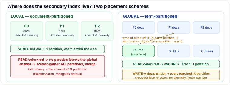
Two placement schemes, mechanism-first
- Local / document-partitioned index — each partition maintains an index that covers only the documents that already live there. A write touches exactly the doc's own partition, so the index update is atomic with the write itself — no coordination with any other node. But no single partition knows the global answer to "which docs have color=red," because red cars might be scattered across all of them. A query on the secondary key must be sent to every partition (scatter-gather), each does a cheap local lookup, and the results are merged at the querying node. Cost grows with partition count, and latency is bounded by the slowest partition, not the average. This is the default in Elasticsearch/Solr (each shard's own Lucene segment only indexes its own documents) and MongoDB.
- Global / term-partitioned index — the index is partitioned independently of the documents, by the indexed term (the value being searched, e.g. the color) rather than by document id. All "color=red" entries live together on one (or a small number of) index partition(s), so a read for that term is routed straight to the owning partition — no scatter, no merge. The cost moves to the write side: a single document write may now touch the document's own home partition plus one index partition per distinct indexed value it has — different physical partitions, often different nodes. Because a single write can no longer be a local atomic operation across all of them, systems typically apply the index-side updates asynchronously (a background job or replication stream), which means the global index is eventually consistent: a read immediately after a write can miss it, and a crash mid-update can leave the index and the documents disagreeing until repaired. DynamoDB Global Secondary Indexes and Riak/Cassandra secondary indexes work this way.
Traced example: color=red over 6 partitions
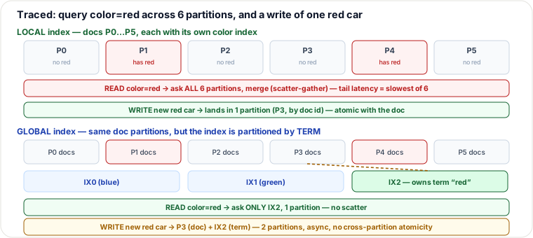
Take 6 partitions P0…P5. Two of them, P1 and P4, happen to hold documents with color=red — "happen to," because documents are placed by their own id, with no relationship to color. Now run the query color=red and a write of one new red car under each scheme.
| Operation | Local (document-partitioned) | Global (term-partitioned) |
|---|---|---|
Read color=red | ask all 6 partitions, merge — 6 requests, tail latency = slowest of 6 | ask only the partition owning term "red" (here IX2) — 1 request |
| Write a new red car | 1 partition (the doc's own, e.g. P3) — atomic with the write | 2+ partitions: P3 (the doc) and IX2 (the "red" term) — cross-partition, usually async |
The asymmetry is the entire lesson: local pays the fan-out cost on every read of the secondary key, no matter how rare that query is. Global pays a smaller, bounded fan-out on every write that touches an indexed field, and in exchange gives every secondary-key read a single-partition, low-latency path. Neither scheme changes what the primary-key partitioning does — both still route by id for document storage; they differ only in where the color→doc mapping lives.
Pitfalls
- Treating local scatter-gather as free. It is N parallel requests per query, and tail latency is the slowest partition's, not the average — a single slow or GC-paused partition drags down every secondary-key query, even ones that touch it by coincidence.
- Assuming a global index write is atomic or synchronous. It almost never is. Right after a write, a read via the secondary index can return stale or missing results until the async index update lands — a real eventual-consistency window, not a hypothetical one.
- Hot terms in a global index. A single very common value (a popular color, a default status) concentrates load onto whichever partition owns that term, recreating the exact hotspot problem sharding was supposed to solve — the fix is the same as for any hot key: sub-partition or salt the term.
- Orphaned global-index entries after a partial failure. If the process crashes after writing the document but before the index-side update lands (or vice versa), the index can point at data that moved or no longer exists until a repair/rebuild job runs.
- Calling local scatter-gather a "distributed transaction." It isn't one — it's independent local reads merged by the coordinator. If one partition is down, you get an incomplete or erroring result unless the caller explicitly handles partial failures.
Selection & trade-offs — how a senior engineer decides
Ask which side of the secondary-key traffic is heavier: writes on indexed fields, or reads by the secondary key? That single question almost always settles it, because the two schemes just move the fan-out cost from one side to the other — neither eliminates it.
| Scheme | Choose when | Avoid when | Write cost | Read cost |
|---|---|---|---|---|
| Local (document-partitioned) | write-heavy; secondary-key queries are rare, low-selectivity, or batch/analytical (search indexes, log stores) | secondary-key point lookups are frequent and latency-sensitive | 1 partition, atomic | N partitions, scatter-gather, tail-latency bound |
| Global (term-partitioned) | read-heavy point lookups on the secondary key (e.g. "orders by customer_id" as a GSI) | writes must be atomic/synchronous across the record and its indexes; index staleness is unacceptable | doc partition + every touched term partition, usually async | 1 (or few) partition(s) |
There is a third, often-overlooked alternative worth naming: don't index at all — denormalize into a separate table/materialized view keyed directly by the value you query (a CQRS-style read model, e.g. a cars_by_color table populated by a stream). It buys the same single-partition read as a global index, without a shared "index" abstraction lagging behind — but you now own the duplication and the update pipeline yourself, and it has the same async-propagation hazard as a global index, just made explicit in your own code instead of hidden in the database. Crisp rule of thumb: write-heavy or rarely-queried secondary key → local (pay the scatter-gather only when it's actually invoked); read-heavy point lookups on a secondary key → global (pay a bounded write fan-out to make every such read cheap); if the caller needs read-your-own-write on that secondary key, treat the global index's lag as a hazard to design around — read from the primary path, poll, or accept the window — rather than assuming the database made it disappear.
Takeaways
- Partitioning a secondary index is a separate decision from partitioning by primary key — the same dataset needs both.
- Local (document-partitioned): cheap, atomic writes; reads on the secondary key must scatter-gather every partition, with tail latency set by the slowest one.
- Global (term-partitioned): reads on the secondary key hit one partition; writes fan out across the doc partition and every touched index partition, usually asynchronously — no cross-partition atomicity, and the index can lag.
- Decide by which side of the traffic is heavier — write-heavy/rare-query → local; read-heavy point-lookup → global — or sidestep the trade-off entirely with an explicit denormalized read model.
Re-authored for this guide; both diagrams hand-authored as SVG. Source: Martin Kleppmann, Designing Data-Intensive Applications, ch. 6 (Partitioning and Secondary Indexes) — the document-partitioned vs term-partitioned distinction and the Elasticsearch/MongoDB/DynamoDB examples are drawn from that chapter. See also: Sharding Strategies (range vs hash vs directory vs geo).
🤖 Don't fully get this? Learn it with Claude
Stuck on Secondary Indexes in Partitioned Systems: local vs global? Open Claude, copy a block below, and it'll teach you this exact concept — visually and interactively.
Build the mental picture, not memorization.
I just read a lesson on **Secondary Indexes in Partitioned Systems: local vs global** (System Design) and want to truly understand it. Explain Secondary Indexes in Partitioned Systems: local vs global from first principles using ONE vivid real-world analogy and a visual mental model — draw it as ASCII art or a clear step-by-step diagram — with a concrete example using real numbers. Then ask me one question to check I got the mental picture, and wait for my reply. If you're unsure or a claim isn't standard, say so and reason from first principles instead of guessing.
Socratic — adapts to where you're stuck.
Teach me **Secondary Indexes in Partitioned Systems: local vs global** interactively. Ask me ONE guiding question at a time, wait for my answer, and adapt to my confusion — build the idea with me step by step instead of explaining it all at once. If you're unsure or a claim isn't standard, say so and reason from first principles instead of guessing.
Active recall exposes what you missed.
Quiz me on **Secondary Indexes in Partitioned Systems: local vs global** with 5 questions, easy to tricky, ONE at a time. Tell me if each answer is right; at the end, explain clearly what I got wrong and why. If you're unsure or a claim isn't standard, say so and reason from first principles instead of guessing.
Intuition + hook + flashcards for long-term memory.
Help me remember **Secondary Indexes in Partitioned Systems: local vs global** for the long term: give the one-sentence intuition, a memorable hook/mnemonic, a tiny worked example, and 3 active-recall flashcards (Q -> A). If you're unsure or a claim isn't standard, say so and reason from first principles instead of guessing.