Load Balancing Algorithms
A load-balancing algorithm is the decision rule a balancer runs on every incoming request to choose which backend serves it — and the only thing that separates the ten famous algorithms is how much live state about the backends that rule is allowed to consult: nothing at all (a fixed rotation), a client identifier (hashing), or real-time health signals (open connections, latency, bandwidth). Everything below is a point on that spectrum.
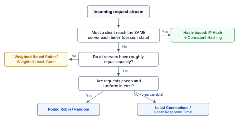
Rather than memorise ten near-identical pros/cons lists, decide with four axes. Almost every real choice falls out of them:
- Homogeneous vs heterogeneous backends. Identical machines can share load blindly; mixed capacity needs weights.
- Stateless vs stateful (session affinity). If a client must keep hitting the same server (in-memory session, local cache), you need a hash, not a rotation.
- Load-blind vs load-aware. Blind rules (Round Robin, Random) are O(1) and need no bookkeeping; load-aware rules (Least Connections, Least Response Time, Least Bandwidth) track per-server metrics and adapt, at the cost of state and oscillation risk.
- L4 vs L7 — where the balancer sits. An L4 balancer sees only TCP/UDP (source IP, port); it is cheap and can do Round Robin, Least Connections, or hash on the 5-tuple, but it cannot read a URL or cookie. An L7 balancer terminates HTTP, so it can route by path/header and pin sessions with a cookie (far more precise than IP hashing), but it burns more CPU per request.
The tree below is the whole page in one picture.
Traced: why "blind rotation" quietly overloads a server
The gap between Round Robin and Least Connections is invisible until request lifetimes differ — which they always do in reality (a file upload holds a connection far longer than a health check). Here is the same stream fed to both, on three identical backends S1, S2, S3.
Setup: six requests arrive one per tick. Two are long-lived (hold the connection open for the rest of the window); four are short (finish inside their own tick). The long ones arrive at tick 1 and tick 4. Least Connections picks the server with the fewest currently-open connections, breaking ties by lowest index.
| Tick | Request | Round Robin picks | Least Connections picks (open counts before) |
|---|---|---|---|
| 1 | R1 (long) | S1 | S1 (0,0,0 → tie, S1) |
| 2 | R2 (short) | S2 | S2 (1,0,0) |
| 3 | R3 (short) | S3 | S2 (1,0,0 → S2 lowest idle) |
| 4 | R4 (long) | S1 ← 2nd long conn! | S2 (1,0,0) |
| 5 | R5 (short) | S2 | S3 (1,1,0) |
| 6 | R6 (short) | S3 | S3 (1,1,0) |
Persistent load left behind:
- Round Robin → S1 = 2 long connections, S2 = 0, S3 = 0. The rotation had no idea R1 was still running, so when the second long request landed on S1's slot in the cycle it doubled up the one server already carrying the heavy load.
- Least Connections → S1 = 1, S2 = 1, S3 = 0. Because S1 still showed an open connection at tick 4, the long request was steered elsewhere. Max load per server: 1 instead of 2.
That is the entire argument for load-aware balancing: identical hardware plus a blind rule still produces a hot server the moment request costs stop being uniform.
The ten algorithms, on one page
Each row is a mechanism plus where it lands on the axes. The families matter more than the names.
| Algorithm | Mechanism (the rule) | Load-aware? | Sticky? | Best when |
|---|---|---|---|---|
| Round Robin | Cyclic: server[i], i = (i+1) mod n | No | No | Homogeneous, stateless, uniform cheap requests |
| Weighted Round Robin | Same, but each server appears in the cycle in proportion to its weight | No (static weights) | No | Heterogeneous hardware, predictable load |
| Random | Pick a server uniformly at random | No | No | Homogeneous; want O(1) with zero shared state (great for many independent balancers) |
| Power-of-two-choices | Sample 2 servers uniformly at random, send to the one with fewer active requests | Yes (samples load) | No | Many independent balancer replicas at scale; want near-LC balance without a global least-loaded structure |
| Least Connections | Fewest currently-open connections | Yes (connections) | No | Long-lived / variable-duration requests |
| Weighted Least Connections | Minimise connections ÷ weight | Yes | No | Heterogeneous and variable load |
| Least Response Time | Lowest recent latency (often × connections) | Yes (latency) | No | Latency-critical services; backends of differing speed |
| Least Bandwidth | Server currently pushing the fewest Mbps | Yes (throughput) | No | Streaming, large downloads, CDNs |
| IP Hash | server = hash(client IP) mod n | No | Yes (by IP) | Need affinity at L4 with no cookie available |
| Custom / metric-based | Weighted score over CPU, memory, queue depth, app metrics | Yes (composite) | Configurable | Standard rules fail; you have a real bottleneck metric to optimise |
Read top-to-bottom, the table is just the spectrum again: static → load-aware → hashed → fully custom, trading simplicity for adaptivity at each step.
Power-of-two-choices sits between Random and Least Connections: it pays two lookups instead of a full scan and, at large n, bounds the maximum load to ~log log n growth instead of log n / log log n for plain random — see the traced companion page for it beating both Round Robin and naive Least Connections on the same request stream.
Why IP-hash breaks on a resize — the road to consistent hashing
IP Hash's appeal is that it needs no state: server = hash(clientIP) mod n deterministically pins a client to a backend. Its fatal flaw is the mod n. Change n — add one server, or lose one to a crash — and nearly every client remaps. Trace four clients across a 3→4 scale-up:
| Client | hash | 3 servers: hash % 3 | 4 servers: hash % 4 | Result |
|---|---|---|---|---|
| C1 | 17 | 2 → S2 | 1 → S1 | moved |
| C2 | 23 | 2 → S2 | 3 → S3 | moved |
| C3 | 18 | 0 → S0 | 2 → S2 | moved |
| C4 | 12 | 0 → S0 | 0 → S0 | stayed |
3 of 4 clients jumped servers by adding a single node. That is not bad luck — plain modulo remaps on the order of (n-1)/n of all keys on any resize. For sticky sessions that means mass logout; for a sharded cache it means a near-total cache flush and a thundering herd onto the origin exactly when you were trying to add capacity.
Consistent hashing fixes this: it places servers and keys on a hash ring, so adding or removing a node only remaps the keys in that node's arc — about 1/n of keys, not (n-1)/n. This is why every serious affinity/sharding system (Cassandra, DynamoDB, memcached clients, Envoy's ring-hash) uses consistent hashing rather than mod n. See the dedicated Consistent Hashing lesson for the ring construction and virtual nodes.
Pitfalls
- Keep-alive poisons Least Connections. HTTP keep-alive and connection pools hold sockets open while idle. A server can show many "open connections" that are doing nothing, so Least Connections starves it while a genuinely busier server keeps getting traffic. Count active requests, not raw sockets, or use Least Response Time.
- IP Hash behind NAT/CGNAT collapses to a hot spot. A whole office, a mobile carrier's CGNAT, or a corporate proxy presents thousands of users as one source IP — all hashing to a single backend. The "even" distribution assumes IP diversity you often don't have. Prefer L7 cookie affinity when you control HTTP.
- Least-Response-Time / Least-Bandwidth oscillation (herding). The moment one server looks fastest, the rule pours all new traffic at it until it slows, then the herd stampedes to the next-fastest — producing sawtooth load. Smooth the metric (EWMA) and/or use "power of two choices" (sample 2 servers, pick the better) to damp it.
- Round Robin on heterogeneous hardware. One weak node in a fleet gets the same share as the beefy ones and saturates first, capping the whole fleet at the weak node's ceiling. Switch to weighted, or autoscale to homogeneous instance types.
- Modulo rehash on scale events (covered above): never use
hash % nfor anything you can't afford to lose on a deploy. - Algorithm can't see "up but sick." A server passing shallow TCP health checks may be GC-thrashing and answering slowly. Blind rules keep feeding it. Pair any algorithm with passive health checks and outlier ejection (temporarily remove a backend whose error/latency spikes).
When to use which — and what it costs
The senior move is to start with the cheapest rule that satisfies your constraints and only climb the spectrum when a real signal forces it.
- Choose Round Robin (or Random) when backends are identical, requests are stateless and roughly uniform, and you want zero coordination. Cost: load-blind — the traced example shows it hot-spots as soon as durations vary. Random additionally needs no shared counter, so it scales across many parallel balancers where Round Robin's shared index would contend.
- Prefer Least Connections when request durations vary (uploads, streaming, slow queries) even on identical hardware. What you gain: automatic avoidance of the pile-up above. Cost: the balancer must track per-server connection state, and it's vulnerable to the keep-alive skew pitfall.
- Prefer Weighted (RR or Least-Conn) the instant your fleet is heterogeneous. Cost: weights are a static guess that drifts as you change instance types; wrong weights are worse than none.
- Prefer Least Response Time when tail latency is the product (trading, gaming, real-time APIs). Cost: most oscillation-prone; needs metric smoothing.
- Prefer hashing only when you genuinely need affinity (in-memory sessions, local cache, sharded stores). Even then, choose consistent hashing over IP-hash/
mod nso scaling doesn't wipe the mapping — and if you speak HTTP, an L7 cookie beats hashing on IP because it survives NAT and client IP changes.
Round Robin vs Least Connections vs Consistent Hashing in one line: Round Robin is free but blind; Least Connections adapts to real load at the price of per-server state; consistent hashing buys you stable affinity at the price of giving up load-awareness entirely. The best real systems layer them — e.g. an L7 balancer doing weighted least-connections within a group, and consistent hashing to pick the group for a sharded key.
Interviewer follow-ups — model answers
- "Why not always Least Response Time?"
Bar: It herds: the momentarily fastest node absorbs all new traffic until it slows, then the herd stampede to the next — sawtooth load unless you EWMA the metric or use power-of-two choices. Prefer Least Connections for variable duration; LRT only when p99 is the product metric and you can damp oscillation. - "We need sticky sessions. IP hash ok?"
Bar: No behind NAT/CGNAT — thousands of users collapse to one IP → one backend. Prefer L7 cookie affinity. If you must hash, use consistent hashing so scale-out remaps ~1/n keys, not (n−1)/n. Also: sticky fights autoscale; prefer external session store when you can. - "Fleet is mixed c5.large and c5.2xlarge — Round Robin fine?"
Bar: No — equal share saturates the small box and caps the fleet. Weighted RR or weighted least-conn with weights ∝ capacity. Better long-term: homogeneous instance types + autoscaling so weights stay trivial.
Takeaways
- The ten algorithms are three families on one spectrum: static (Round Robin, Weighted, Random) → load-aware (Least Connections/Response/Bandwidth) → hashed (IP Hash → Consistent Hashing), trading simplicity for adaptivity.
- Decide with four questions: heterogeneous hardware → weights; sticky sessions → hash; variable request cost → least-connections; can you read HTTP → L7 routing/cookies.
- Blind rotation quietly overloads a server the moment request durations differ — the traced run left Round Robin with 2 long connections on one node while Least Connections spread them 1-and-1.
- Never balance affinity with
hash % n: a single scale event remaps ~(n-1)/nof clients. Consistent hashing remaps only ~1/n— that gap is the whole reason it exists.
Re-authored and deepened for this guide. Sources: NGINX documentation, "Choosing an NGINX Plus Load-Balancing Method"; HAProxy Configuration Manual (the balance directive: roundrobin, leastconn, source, uri); AWS Elastic Load Balancing / Application Load Balancer developer guides (target groups, outlier detection, cross-zone balancing); Envoy proxy load-balancing docs (ring-hash, Maglev, least-request, power-of-two-choices); Karger et al., "Consistent Hashing and Random Trees" (STOC 1997); Alex Xu, System Design Interview, Vol. 1. Worked traces and the decision tree are original to this guide.
🤖 Don't fully get this? Learn it with Claude
Stuck on Load Balancing Algorithms? Open Claude, copy a block below, and it'll teach you this exact concept — visually and interactively.
Build the mental picture, not memorization.
I just read a lesson on **Load Balancing Algorithms** (System Design) and want to truly understand it. Explain Load Balancing Algorithms from first principles using ONE vivid real-world analogy and a visual mental model — draw it as ASCII art or a clear step-by-step diagram — with a concrete example using real numbers. Then ask me one question to check I got the mental picture, and wait for my reply. If you're unsure or a claim isn't standard, say so and reason from first principles instead of guessing.
Socratic — adapts to where you're stuck.
Teach me **Load Balancing Algorithms** interactively. Ask me ONE guiding question at a time, wait for my answer, and adapt to my confusion — build the idea with me step by step instead of explaining it all at once. If you're unsure or a claim isn't standard, say so and reason from first principles instead of guessing.
Active recall exposes what you missed.
Quiz me on **Load Balancing Algorithms** with 5 questions, easy to tricky, ONE at a time. Tell me if each answer is right; at the end, explain clearly what I got wrong and why. If you're unsure or a claim isn't standard, say so and reason from first principles instead of guessing.
Intuition + hook + flashcards for long-term memory.
Help me remember **Load Balancing Algorithms** for the long term: give the one-sentence intuition, a memorable hook/mnemonic, a tiny worked example, and 3 active-recall flashcards (Q -> A). If you're unsure or a claim isn't standard, say so and reason from first principles instead of guessing.