Key Characteristics of Distributed Systems

Overview

A distributed system is judged on five characteristics: Scalability, Reliability, Availability, Efficiency, and Manageability. These aren't independent knobs — pushing on one usually costs you on another (more redundancy for reliability costs money and coordination overhead; more horizontal scaling costs manageability). The rest of this lesson works through each one and, because vague definitions don't transfer to an interview or a design doc, carries the availability and efficiency numbers all the way through with real arithmetic instead of stopping at "just add more nines."

Scalability

Scalability is the capability of a system, process, or network to grow and handle increased demand without a loss of performance. A system may need to scale because of more data, more traffic, or more transactions, and a well-scaled system absorbs that growth without degrading.

In practice, performance usually declines somewhat as a system grows, even in systems designed to scale — coordination overhead rises, network hops get longer, and some tasks resist being split up at all. A well-designed scalable architecture minimizes this decline and spreads load evenly across participating nodes rather than concentrating it.

Horizontal vs. vertical scaling

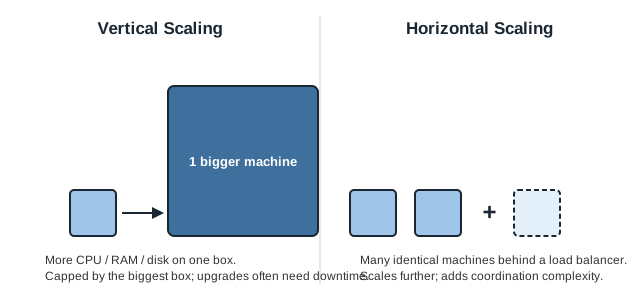
Horizontal scaling means adding more machines to the pool of resources. Vertical scaling means adding more power — CPU, RAM, storage — to an existing machine.

Horizontal scaling is usually easier to do dynamically: you add another box to the pool without touching the ones already running. Vertical scaling is capped by the biggest machine you can buy, and pushing past a machine's current capacity typically means downtime for the upgrade.

Cassandra and MongoDB are commonly cited examples of systems built to scale horizontally — both make it straightforward to add more machines as load grows. MySQL is the classic vertical-scaling example: moving to a bigger box is the standard first move, though it usually costs some downtime to do it.

Reliability

Reliability is a system's ability to keep operating correctly in the presence of faults, errors, or failed components. A distributed system is reliable if it keeps delivering its service even when some of its hardware or software fails, because a failing machine can be replaced by a healthy one without the requester ever noticing.

Take a large e-commerce store: a core requirement is that a user's transaction, or their shopping cart, should never be lost just because the machine handling it crashed. A reliable system achieves this through redundancy of both software and data — if the server holding a cart fails, a replica takes over. That redundancy isn't free: a reliable system has to pay its cost in hardware, replication traffic, and coordination in exchange for eliminating single points of failure.

Reliability vs. fault tolerance

Fault tolerance is a closely related but narrower idea: it is the property that lets a system keep operating, possibly in a degraded mode, when one or more components fail — the mechanism, not the outcome. Reliability is the broader, user-facing outcome that fault tolerance helps produce.

• Scope — Reliability is about the end-to-end correctness and consistency of the whole system over time; fault tolerance is about whether the system keeps running when an individual component fails.
• Perspective — Reliability is user-centric: does the system keep meeting the user's expectations? Fault tolerance is system-centric: how does it handle internal breakdowns?
• Measurement — Reliability is typically measured with uptime, error rates, or mean time between failures (MTBF). Fault tolerance is measured by how fast and cleanly the system detects, isolates, and recovers from a failure — for example, failover time.

Reliability vs. availability, in one example: an online retail store runs at 99.99% availability for two years, but launches without any real security testing. Customers are happy — the system looks fine — but it isn't very reliable, because it's carrying an untested risk. In year three, a string of security incidents causes extended outages: high availability for two years didn't mean the system was reliable, it meant nothing bad had happened yet.

Availability

Availability is the percentage of time a system remains operational and able to do its job, in a given period. It's a narrower measure than reliability: an unreliable product can still post high availability if repairs are fast and spares are always on hand — which is exactly why a system can look fine for years and then take a bad quarter once an underlying risk catches up with it.

Where the numbers come from: MTBF and MTTR

Availability for a single component is usually derived from two numbers: MTBF (mean time between failures — how long it typically runs before breaking) and MTTR (mean time to repair — how long it typically takes to fix once it breaks).

Availability = MTBF / (MTBF + MTTR)

Downtime for a given period (say, a year, 8,760 hours) = MTTR / (MTBF + MTTR) × 8,760 hours.

Worked example: a three-tier request path

Suppose a request passes through a load balancer, an application server, and a database, in series — if any one of them is down, the request fails. Take these specs:

• Load balancer — MTBF 9,999 h, MTTR 1 h → availability = 9,999 / 10,000 = 99.99%, downtime ≈ 0.876 h/yr.
• Application server — MTBF 999 h, MTTR 1 h → availability = 999 / 1,000 = 99.9%, downtime ≈ 8.76 h/yr.
• Database — MTBF 1,999 h, MTTR 1 h → availability = 1,999 / 2,000 = 99.95%, downtime ≈ 4.38 h/yr.

Because the three sit in series, the path's overall availability is the product of the three, not the average and not just the weakest one:

0.9999 × 0.999 × 0.9995 = 0.998401 → 99.8401%, which rounds to 99.84%.

That's lower than the weakest individual link (the app server, at 99.9%) — series composition always compounds downward. In hours: (1 − 0.998401) × 8,760 h ≈ 14.01 hours of downtime a year for the whole path, even though no single component looks that unreliable on its own. This is the "weakest link" idea in its precise form: a chain's availability isn't bounded by its weakest link, it's strictly worse than its weakest link.

A precision aside, on its own numbers

Here is a separate, self-contained example — not connected to the load balancer / app / database numbers above — chosen specifically to expose a common arithmetic mistake. Suppose a component has MTBF = 720 hours and MTTR = 2 hours. Its exact availability is 720 / 722 = 99.7230%. If you round that to 99.72% for display and then estimate downtime as (100% − 99.72%) × 8,760 h = 0.28% × 8,760 h ≈ 24.53 hours/year, you've introduced an avoidable error: the true figure, computed straight from the exact ratio, is 2 / 722 × 8,760 h ≈ 24.27 hours/year. The gap is roughly a 1% relative error — on the order of fifteen minutes a year — which looks negligible in isolation, but it's exactly the kind of rounding cascade that compounds silently once you start multiplying several such figures together across a multi-tier chain. Rule of thumb: carry full precision through every multiplication, and only round the very last number you display.

Worked example, continued: adding redundancy

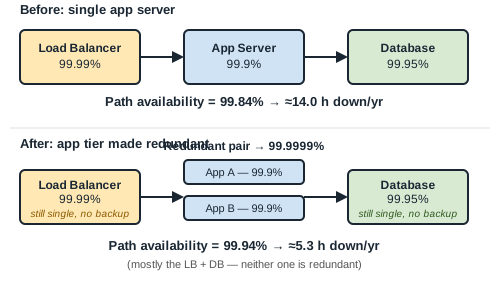
Back to the load balancer / app server / database path above. The application tier, at 99.9%, is the weakest of the three. Suppose we add a second, identical app server running active-active behind the same load balancer, and assume — for now — that the two fail independently. A single app server is unavailable 0.1% of the time (1 − 0.999 = 0.001); for the pair to be down, both have to be down at once:

Pair unavailability = 0.001 × 0.001 = 0.000001 → pair availability = 99.9999%, downtime ≈ 0.0088 h/yr — about half a minute a year.

Recomputing the whole path with the redundant app tier in place:

0.9999 × 0.999999 × 0.9995 = 0.999399 → 99.9399%, which rounds to 99.94%, or about 5.26 hours of downtime a year — down from 14.01 hours, but nowhere near the 99.9999% the app tier alone now boasts.

The reason is the "weakest link" principle again, just relocated: with the app tier's contribution reduced to a rounding error, the remaining ~5.26 hours of yearly downtime is now almost entirely the load balancer's 0.876 hours and the database's 4.38 hours — two links that were never touched. Redundancy at one tier doesn't raise the ceiling set by the tiers you didn't redouble.

Efficiency

Efficiency asks how cheaply a distributed operation delivers its result. Two standard measures: response time (or latency) — the delay until the first item comes back — and throughput (or bandwidth) — how many items are delivered per unit time. Those two measures map onto two unit costs:

• Number of messages sent globally by the nodes of the system, regardless of message size.
• Size of messages, representing the volume of data actually exchanged.

Analyzing a distributed data structure purely by "number of messages" is a deliberately crude simplification — it ignores network topology, load variation, and hardware/software heterogeneity. It's a useful first cut precisely because a fully accurate cost model is hard to build; you trade precision for a number you can actually compute and compare. Here is what that first cut looks like with real numbers, rather than left as an abstraction.

Concrete comparison: two-phase commit vs. quorum, at N = 5

Take a 5-node replicated system and compare two ways of durably committing a write.

Two-phase commit (all-node agreement). A coordinator drives commit across the other 4 replicas. Phase 1 (prepare): 4 messages out, 4 votes back = 8. Phase 2 (commit): 4 messages out, 4 acks back = 8. Total: 16 messages for one write — and it doesn't complete until every one of the 5 nodes has responded twice, so one slow or dead node stalls the whole operation.

Quorum write (W = 3 of N = 5). The coordinator only needs 2 more acknowledgments to reach a write quorum of 3 (itself plus 2). The messages that sit on the latency-critical path are 2 requests out and 2 acks back: 4 messages. The other 2 replicas still get the write in the background, but the operation doesn't wait on them.

Generalizing: two-phase commit costs 4 × (N − 1) messages and blocks on the slowest of all N nodes; a quorum write with quorum size W costs 2 × (W − 1) messages on the critical path and blocks on the slowest of only W nodes. At N = 5, W = 3, that's 16 versus 4 — a 4x difference in message count for a comparable durability guarantee, before message size, network topology, or hardware differences enter the picture at all. That's also part of why quorum-style protocols tolerate node failure and scale better than all-node consensus for the same read/write pattern: fewer messages on the path that determines latency, and fewer nodes that have to be alive for the operation to succeed.

None of this replaces a real cost model — it still says nothing about payload size, cross-region hops, or a node that's alive but slow — which is exactly why it's called a first cut, not the whole story. But it is concrete enough to compare two designs on paper before building either one.

Serviceability, or Manageability

Another important consideration is how easy a system is to operate and maintain. Serviceability (or manageability) is the simplicity and speed with which a system can be repaired or maintained — since time-to-fix feeds directly into availability, a system that's hard to diagnose or patch will have worse availability even if its raw MTBF is fine.

Things worth checking here: how easy it is to diagnose and understand a problem when one occurs, how easy it is to ship an update or a fix, and how much the system runs on its own without routine hand-holding. Early fault detection matters too — some systems automatically page or open a ticket the moment a fault is detected, shrinking MTTR before a human has even looked at it, which, per the MTBF/MTTR formula above, directly buys back availability.

Pitfalls

Two mistakes are common enough, and costly enough, to call out explicitly — both hiding inside the redundancy worked example above.

1. Treating failures as independent when they aren't

The parallel-redundancy calculation above — squaring 0.1% unavailability down to 0.0001% — is only valid if the two app server instances fail independently. That assumption is the single most common thing designers get wrong about redundancy. If both instances share a power feed, a rack, a network switch, an availability zone, or simply receive the same bad config push or the same buggy deploy at the same time, their failures are correlated, not independent — and the "square the unavailability" shortcut collapses back toward the single-node figure of 99.9% available (0.1% unavailable), roughly a 1,000x worse outcome than the 99.9999% the naive math promised. Redundancy only buys the availability the arithmetic predicts if you can point to genuinely separate failure domains — separate power, separate network path, separate rack or AZ, and ideally staggered deploys — for every replica you're counting as "independent."

2. Adding redundancy behind a single load balancer — or in front of a single database

Adding redundancy behind a single load balancer, or in front of a single un-replicated database, doesn't remove a single point of failure — it just relocates it. In the worked example above, doubling the app tier improved that link from 99.9% to 99.9999%, but the overall path only moved from 99.84% to 99.94%, because the load balancer (99.99%, 0.876 hours of downtime a year on its own) and the database (99.95%, 4.38 hours a year) were never touched — and neither one has a backup. If that single load balancer goes down, it doesn't matter that two healthy app servers are sitting behind it: the entire path is unavailable. Any redundancy pass that stops at one tier without asking "what's still single-homed upstream and downstream of the thing I just fixed?" has moved the bottleneck, not eliminated it — and in this example, the database is now the largest single contributor to the path's remaining downtime (4.38 of the 5.26 hours a year), which is exactly where the next round of redundancy work should go.

The distributed-systems tax: partial failure, unbounded latency, no global clock

Three realities sit underneath every characteristic above and explain why distributed systems need timeouts, retries, and consensus in the first place. Partial failure means some components are down or slow while others keep accepting work — unlike a single process, which is either up or down, a distributed system is normally in some mixed state. Unbounded latency means a call that is merely slow is indistinguishable from one that will never return, so you cannot wait forever: a blocked caller holds a thread and a connection, and enough of them hang the whole fleet. No global clock means wall-clock timestamps cannot be trusted to order events across machines — NTP skew alone can reorder them — which is why causality is tracked with logical clocks or version vectors rather than System.currentTimeMillis().

The interaction of the first two produces retry amplification, worth quantifying because it is how a healthy cluster tips into collapse. Suppose each RPC has a 200 ms timeout and a retry budget of 2 (three attempts total): a request that keeps timing out waits up to 200 × 3 = 600 ms before giving up. Now put that under load — 5,000 QPS with a 2% timeout rate: 5,000 × 0.02 = 100 timeouts/s, each retried twice = +200 backend calls/s, a 4% traffic amplification aimed squarely at the tier that is already struggling. On a near-saturated cluster that extra 4% is often what turns a brownout into an outage. The bound is the standard resilience kit: finite timeouts, retry budgets (not unlimited retries), backoff with jitter, and circuit breakers that stop hammering a tier that is already failing. Do not import any of this machinery where it does not belong: a single-process batch job has none of these problems and needs none of these mechanisms.

Sources

Core definitions and terminology (scalability, reliability, availability, efficiency, serviceability) follow the standard treatment used across mainstream system-design interview references, notably Design Gurus' Grokking the System Design Interview and similar system-design-primer style material. The MTBF/MTTR availability formulas are standard reliability-engineering definitions found throughout the site-reliability-engineering literature (e.g. Google's SRE book). The quantitative worked examples in this deepened treatment — the three-tier chain and redundancy arithmetic, the rounding-cascade illustration, and the two-phase-commit-versus-quorum message-count comparison — were composed for this page to make the "do the math" claims in the original lesson concrete and independently checkable.