Building Blocks II — gRPC/GraphQL/REST at Scale, Geospatial Indexing (Geohash/S2/H3) & N-tier Trade-offs (Deep Dive)

Five building blocks that keep resurfacing once a design gets specific about its API layer, its geo-query layer, and its deployment topology. Each one has the same shape of gotcha: a mechanism that is efficient exactly because it hides state (one TCP connection, one resolver call, one shard key, one field number) — and that hidden state is precisely what breaks under scale if you don't know it's there.

1. gRPC over an L4 load balancer — the connection-pinning gotcha

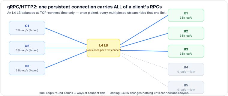
gRPC runs on HTTP/2, and HTTP/2's whole efficiency trick is multiplexing: a client opens one TCP connection and rides it for thousands of concurrent RPCs, each its own logical stream inside that one connection, kept alive indefinitely instead of reconnecting per call (the way HTTP/1.1 effectively did). A load balancer that operates at L4 (TCP/connection level — e.g. a plain network load balancer) makes its balancing decision exactly once: at the TCP handshake. After that, the LB is just forwarding bytes on an established pipe — it never looks inside the connection again. So every RPC stream multiplexed over that one connection, for the entire lifetime of the client process, lands on the same backend it happened to get at connect time.

Traced example — 3 clients, 5 backends, one L4 round-robin

Three client pods (C1, C2, C3) each start up and open one long-lived gRPC channel to the service's L4 LB. The LB round-robins the three TCP handshakes across five backend pods (B1–B5): C1 → B1, C2 → B2, C3 → B3. Traffic then ramps to 100k req/s, split evenly across the three clients (33k req/s each) — but every one of those requests is just another stream multiplexed onto the connection its client already holds.

Client	Connection made once to	Requests carried (any volume)
C1	B1	33k req/s, forever, until reconnect
C2	B2	33k req/s, forever, until reconnect
C3	B3	33k req/s, forever, until reconnect
—	B4, B5	0 req/s — never chosen, connections already fixed

Round-robin "worked" at connect time — each of the first three connections went to a different backend — but the result is a 100%-vs-0% imbalance at the request level, and it is permanent: scaling the backend fleet from 5 pods to 50 changes nothing, because no new TCP connection is ever made until an existing one drops.

The fix

• L7 (request-level) load balancing. An L7-aware proxy (Envoy, a service-mesh sidecar, an ALB/gateway with HTTP/2-aware routing) terminates the client's HTTP/2 connection and re-distributes each individual stream across its own pool of connections to the backends — the balancing unit becomes the RPC, not the TCP connection.
• Client-side load balancing. The gRPC client itself resolves multiple backend addresses (via DNS SRV records or an xDS control plane) and opens several connections, picking one per RPC (gRPC's round_robin or pick_first policies) — no proxy needed at all.
• Connection recycling. Setting MAX_CONNECTION_AGE (and MAX_CONNECTION_AGE_GRACE) server-side forces a periodic GOAWAY, making the client reconnect and re-run the LB decision — a coarse, time-smeared mitigation on top of a dumb L4 LB, not a real fix by itself.

Pitfalls

• "We're using round-robin" is not the same claim at the connection level as at the request level — always ask which unit the LB balances.
• A newly added backend can sit at 0 req/s indefinitely if existing clients never reconnect; health checks that only probe TCP reachability won't catch this — you need request-rate-per-backend metrics.
• Naive fix "just restart the clients periodically" is exactly what MAX_CONNECTION_AGE automates server-side — prefer the explicit knob over ad hoc client bouncing.

2. GraphQL's N+1 resolver explosion — and why DataLoader batches it away

A GraphQL executor resolves a query field by field, and each field resolver is written as if it were the only thing running — it has no visibility into its siblings. Take:

{
  posts {          # resolver: SELECT * FROM posts LIMIT 20      (1 query)
    id
    title
    author {       # resolver: SELECT * FROM users WHERE id = ?  (called once PER post)
      name
    }
  }
}

The posts resolver runs once and returns 20 posts. The author resolver then runs once per post in the list, because that's the only unit the executor gives it — 20 independent calls, each doing its own point lookup. Total: 1 (posts) + 20 (authors) = 21 queries for data that a single WHERE id IN (...) could have fetched in 2. That's the N+1 problem, and it's not a bug in any one resolver — it's the default consequence of resolvers being independent functions.

DataLoader: batch on the tick, not the call

DataLoader wraps the per-item load call so it doesn't fire immediately. Each loader.load(authorId) call just queues that key and returns a pending promise; DataLoader waits until the end of the current event-loop tick (a microtask boundary — after all 20 synchronous .load() calls from the 20 author resolvers have already been queued), then fires one batch function, batchLoadAuthors([id1, id2, ..., id20]), and fans the single result set back out to the 20 waiting callers by key. N+1 becomes 2 total round trips — 1 for posts, 1 batched call for every author needed — regardless of how large N grows.

The caching consequence

DataLoader also memoizes: a second .load(sameId) within the same request returns the already-cached promise instead of re-queuing it. But that cache is instantiated fresh, per request (a new DataLoader instance per incoming GraphQL operation) — deliberately, so one user's cached data can never leak into another user's response. It is not a cross-request cache. If you need data to survive past one request, that's a separate layer (Redis, an in-memory LRU with its own invalidation) — DataLoader only solves the *within-one-query* duplicate-fetch problem.

Why GraphQL complicates HTTP caching

REST gets HTTP caching almost for free: GET /posts/42 is a distinct, cacheable URL that a CDN or browser cache can store and reuse. GraphQL, by contrast, almost universally exposes a single endpoint (POST /graphql) with the actual query and variables carried in the request body — and intermediary caches key on URL (and rarely cache POST responses at all), so that free caching layer disappears. The common mitigations are persisted queries (the client sends a hash id instead of the full query text, which can then ride as a GET with the hash in the URL — restoring cacheability) or a bespoke response cache keyed on a hash of (query + variables) instead of the URL.

Pitfalls

• Adding DataLoader doesn't remove the need to think about query shape — a deeply nested query can still fan out into many batches, one per nesting level, even though each level itself is now O(1) queries.
• Forgetting to scope DataLoader per-request (e.g. accidentally sharing one instance across requests for "performance") reintroduces the exact cross-user leak the per-request cache exists to prevent.
• Persisted queries shift the caching win to whichever clients pre-register queries — ad hoc/exploratory querying (GraphiQL, dynamic clients) doesn't benefit.

3. Geospatial indexing: Geohash, S2, and H3

The mechanism behind Geohash: take a point's latitude and longitude, recursively bisect each range (does the point fall in the top or bottom half of the current lat range? left or right half of the current lon range?), and interleave the resulting bits — lon bit, lat bit, lon bit, lat bit, … — into one binary string. Encode every 5 bits of that string as one base-32 character. The payoff: two points that are near each other usually share a long common prefix, which means "find things nearby" becomes a plain string-prefix / range query — the kind any ordinary sorted index (a B-tree, a KV store's range scan) already supports, with no special 2-D index structure needed.

The hot-shard problem

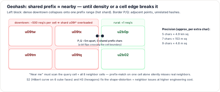
Diagram above, left block: if you partition a datastore by geohash-prefix ranges (common in a range-partitioned KV store), the partition boundaries follow the grid, not the data density. A dense downtown — all of it — can fall inside one or two geohash prefixes, because Geohash bins by fixed lat/lon cell, irrespective of how many points live in that cell. Every check-in, ride request, or delivery order from that block lands on the same one or two shard ranges (u09t* in the diagram) while a same-sized rural cell (u2b0*) sits nearly idle — a classic hot partition produced by a spatially skewed key, not by anything wrong with the partitioning logic itself.

Mitigations: salt the key (append a hash suffix and fan a query out across the salted variants), partition on a coarser prefix than you index on (spreads the hot region across more shard ranges while keeping fine-grained range queries inside each), or decouple the partitioning tier from geographic ordering entirely (consistent hashing for placement, Geohash only for the in-partition range query).

The edge / neighbor-cell problem

Diagram above, points P and Q: two points a few meters apart can sit on opposite sides of a grid boundary where a high-order interleaved bit flips — and when a high bit flips, the resulting prefix can diverge completely, even though the points are practically touching (u09tx next to u2b0p in the diagram, zero shared prefix characters). A naive "prefix-match the query cell" search silently misses real neighbors sitting just across such a boundary. The fix is mechanical, not probabilistic: derive the cell's bounding box from its hash, compute the 8 adjacent bounding boxes by shifting one cell-width in each compass direction (bit manipulation on the interleaved integer, not string surgery), re-encode each to get the 8 neighbor hashes, and search the query cell plus all 8 neighbors. Precision scales with hash length — roughly, each extra character shrinks the cell by about 32× (2^5) in area (approximate standard figures: 5 characters ≈ a 4.9 km cell, 7 characters ≈ a 153 m cell, 9 characters ≈ a 4.8 m cell) — so length is also how you choose search radius.

S2 — Hilbert-curve cells (Google)

S2 projects the sphere onto the 6 faces of a circumscribed cube, then subdivides each face using a Hilbert space-filling curve into a hierarchy of cells, each identified by a single 64-bit cell ID that encodes both position and level. A Hilbert curve preserves spatial locality far more consistently than lat/lon bit-interleaving does — points near each other in space are reliably near each other in the 1-D ordering, so the boundary-flip edge case above is far rarer, and cell area stays near-uniform even close to the poles (Geohash cells distort badly there because lat/lon degrees don't correspond to constant distance). The cost is real engineering overhead — no plain string-prefix trick, you need the S2 library — in exchange for accurate distance math and clean region "coverings" (approximating an arbitrary polygon with a set of S2 cells).

H3 — hexagonal cells (Uber)

H3 tiles the globe with hexagons (built from an icosahedron projection) across 16 resolutions. The property a hexagon has that a square/Geohash cell doesn't: uniform distance to all six neighbors — a square cell is closer to its 4 edge-neighbors than its 4 diagonal-neighbors, a directional bias that quietly distorts anything built on "distance to neighbor" (flow analysis, supply/demand aggregation, k-ring queries). That uniformity is exactly why Uber built it for ride-hailing supply/demand grids. Trade-off: hexagons don't subdivide evenly (a parent hex doesn't split into same-shaped child hexes the way a square or S2 cell splits into 4), and a sphere can't be tiled purely in hexagons — 12 pentagon distortions are unavoidable at the icosahedron's vertices.

Pitfalls

• Treating Geohash prefix-match as a complete "nearby" query without the 8-neighbor scan — the single most common Geohash bug.
• Partitioning a datastore directly on raw Geohash prefix without checking density first — the hot-shard failure is invisible until a real city's worth of traffic hits it.
• Assuming precision (hash length) is uniform in both dimensions — Geohash cells are rectangular, not square; length-to-distance is an approximation, not an exact radius.

4. API versioning & compatibility across REST, gRPC, and GraphQL

REST

Versioned explicitly, in a place the client controls: the URL (/v1/users → /v2/users) or a header (Accept: application/vnd.api+json;version=2). Simple and visible, at the cost of the server maintaining N versions of the same logic (or a translation layer) until old versions are deprecated.

gRPC / protobuf

Wire compatibility is governed by field numbers, not names or declaration order:

message User {
  string name = 1;
  int32 id    = 2;
  // string nickname = 3;   // removed — number 3 must be marked reserved, never reused
  reserved 3;
  string email = 4;         // safe: new field, new number, optional by default in proto3
}

Never reuse or renumber a field number once any client has shipped against it — an old binary reading "field 3" will silently misinterpret whatever new meaning field 3 now carries; this is silent data corruption, not a visible error. New fields are added as new numbers (optional/has-presence by default), so old clients simply ignore fields they don't recognize (forward compatible) and new clients see defaults for fields an old server never sent (backward compatible). This lets one proto service evolve for years without ever needing a /v2 service, as long as changes stay additive.

GraphQL

No version number by convention — the schema evolves additively. Clients ask only for the fields they want, so adding a field or type is inherently non-breaking. Retiring a field goes through @deprecated(reason: "...") — it still resolves, tooling warns callers to migrate — and is only removed once usage analytics confirm nothing still queries it. Versioning is replaced by a deprecation-and-usage-data gate.

Rate-limit store-down behavior (cross-ref: rate limiting / token bucket)

A centrally shared limiter (token bucket or sliding-window counter kept in Redis, per the rate-limiter page in this guide) has one more failure mode worth naming explicitly: what happens when that shared store itself is unreachable?

• Fail-open — treat "can't check the limit" as "allow the request." Preserves availability of the underlying service, but during the outage there is effectively zero rate-limiting protection — risky precisely when the store went down because of the overload the limiter exists to catch.
• Fail-closed — treat "can't check" as "reject." Fully protects the backend, but now an outage in a peripheral component (the limiter store) takes down the entire primary API alongside it.
• Common compromise — fail-open with a local fallback: each instance runs a coarse in-memory token bucket used only while the shared store is unreachable. Less precise (per-instance instead of global) but avoids both full lockout and zero protection.

The token-bucket refill itself is normally computed lazily, blending the last stored state with real elapsed time rather than running a background timer: tokens(t) = min(capacity, tokens_stored + rate × (t − t_last)); a request of cost c is allowed iff tokens(t) ≥ c, after which tokens and t_last are written back. Because that formula reads wall-clock time t on whichever server evaluates it, clock skew across app servers distorts the effective limit: an instance whose clock runs ahead computes a larger elapsed delta and over-refills (quietly raising the limit), one whose clock lags under-refills (quietly throttling below the intended limit). The fix is to source t from one authoritative clock — e.g. Redis's own TIME command evaluated inside the same Lua script that does the check-and-decrement — rather than trusting each caller's local clock.

5. N-tier vs microservices — a two-sided trade-off

	Gains	Costs
N-tier	In-process calls between layers; one deploy pipeline; ACID transactions across "modules" are trivial (one database); simple to reason about one call stack end to end	Whole tier scales as a unit even if only one code path is hot; a leak/crash in one module can take the whole process down; many teams sharing one codebase/deploy slows velocity at scale
Microservices	Independent scaling of exactly the hot service; independent deploy cadence per team; failure isolation (one service crashing doesn't directly crash another); freedom to pick per-service tech	In-process calls become network calls — new failure modes (partial failure, latency, retries); no more free cross-service ACID (sagas / eventual consistency instead); real operational load (service discovery, distributed tracing, the versioning discipline from §4 now applies between your own services)

Decision rule

Default to N-tier/monolith until there is a measured reason to split out a service — a sub-system with a genuinely different, observed scaling profile, a team-ownership boundary causing real coordination pain, or a component that needs its own deploy cadence or tech stack. Split along observed hot spots and organizational boundaries (Conway's law), not guessed future ones — a premature split pays the full distributed-systems tax before any scaling benefit exists to offset it.

The stateless-tier precondition

Horizontally scaling any tier — adding instances behind a load balancer — requires that tier be stateless across requests: no request may depend on in-memory state that exists only on the one instance that handled an earlier request for that client. If it does, the LB must pin that client to that instance (sticky sessions) — the same connection-pinning failure mode as §1, now expressed as session affinity instead of a TCP connection: the client's traffic is bound to one instance instead of freely distributed. The fix is the same shape too: externalize the state (a shared session store, a shared cache) so any instance can serve any request.

Cross-tier failure behavior

Scaling one tier without its downstream dependency keeping pace makes things worse, not better: more app instances generate more concurrent load toward the same database tier, exhausting its connection pool; requests then either queue under back-pressure or get retried — and retries from every app instance amplify load on a database that is already struggling, while clients retrying their own failed calls add a second layer on top. That's a retry storm / cascading failure, and the standard defenses are back-pressure (bounded queues and connection pools that shed load instead of queuing it unboundedly), circuit breakers (stop calling a failing dependency and fail fast instead of retrying into it), and bounded, jittered retry policies (never unbounded retry). Any tier you scale needs an explicit failure/back-pressure contract with its neighbors, or scaling it just moves the bottleneck downstream and adds retry amplification on top.

Judgment layer

L4 vs L7 for gRPC

L4 is cheaper — no per-request parsing, and it works for arbitrary TCP traffic, not just HTTP — and it is fine for traffic patterns that reconnect often (classic HTTP/1.1 request/response). It is the wrong default for gRPC specifically because of connection pinning (§1), unless paired with client-side load balancing or aggressive MAX_CONNECTION_AGE recycling. L7 (a real proxy or mesh sidecar) correctly balances per RPC, and you typically want one anyway if you also want retries, circuit-breaking, or per-request observability at the RPC level — the cost is an extra hop and more CPU spent parsing HTTP/2 frames. Decision: any gRPC service sitting behind a shared LB in production should default to L7 or client-side balancing; reach for pure L4 only for a small, fixed set of long-lived server-to-server links where you control both ends and actively tune connection age.

Geohash vs S2 vs H3

Geohash: pick it when you want a plain string-prefix index inside a KV/SQL store you already have, and you can mitigate hot-shard and neighbor-edge cases directly. S2: pick it when you need accurate distance/region math — "is this point inside this service-area polygon," map-tile-style coverage — and can afford a dedicated geometry library. H3: pick it when the workload is about aggregating or analyzing flow/density uniformly in every direction — supply/demand grids, geo ML features, hex-binned visualizations — where directional uniformity matters more than a simple string key.

REST vs gRPC vs GraphQL

REST: public/partner-facing APIs, browser- and curl-debuggable, gets HTTP caching for free from distinct resource URLs. gRPC: internal service-to-service calls where you control both ends and want low-latency binary framing, strict typed contracts, and streaming — a poor fit for direct browser clients without a gateway. GraphQL: client-driven fetching where the front end composes data from many backend resources in one round trip with exactly the fields it needs — at the cost of HTTP cacheability (§2) and a resolver-complexity risk (N+1) that must be actively managed; strongest when many different client shapes (web, mobile, partner) share one backend graph, weaker for a narrow, stable, single-consumer API where REST's simplicity wins outright.

Takeaways

• Anything that multiplexes many logical units over one long-lived connection (gRPC/HTTP2) breaks connection-level (L4) load balancing — always ask whether your LB decides per-connection or per-request.
• N+1 is the default behavior of independent field resolvers, not a bug in any one of them — batching (DataLoader) is the fix, and its cache is per-request by design, not a substitute for a real cross-request cache.
• A geo-index's cell shape determines what breaks at scale: Geohash breaks on density skew and cell edges; choose the shape (square-prefix, Hilbert/S2, hexagonal/H3) that matches whether you need simple storage, precise region math, or uniform-neighbor analysis.
• Each protocol's compatibility rule follows from what identifies a field on the wire: gRPC's field number is sacred and never reused; REST's version lives explicitly in the URL/header; GraphQL's additive-only contract makes deprecation — not versioning — the actual mechanism.

---

Synthesized from the gRPC load-balancing guide (grpc.io) and Envoy/Google Cloud documentation on L4 vs L7 gRPC balancing; the GraphQL specification's field-resolution semantics and the DataLoader reference implementation (GitHub, graphql/dataloader); Google's S2 geometry library documentation; Uber's H3 documentation; the Protocol Buffers language guide's field-number compatibility rules; Designing Data-Intensive Applications (Kleppmann) on schema evolution and system architecture trade-offs. Cross-references the Rate Limiting and CAP Theorem pages in this guide. Re-authored/Deepened for this guide.

I just read a lesson on **Building Blocks II — gRPC/GraphQL/REST at Scale, Geospatial Indexing (Geohash/S2/H3) & N-tier Trade-offs (Deep Dive)** (System Design) and want to truly understand it. Explain Building Blocks II — gRPC/GraphQL/REST at Scale, Geospatial Indexing (Geohash/S2/H3) & N-tier Trade-offs (Deep Dive) from first principles using ONE vivid real-world analogy and a visual mental model — draw it as ASCII art or a clear step-by-step diagram — with a concrete example using real numbers. Then ask me one question to check I got the mental picture, and wait for my reply. If you're unsure or a claim isn't standard, say so and reason from first principles instead of guessing.

Teach me **Building Blocks II — gRPC/GraphQL/REST at Scale, Geospatial Indexing (Geohash/S2/H3) & N-tier Trade-offs (Deep Dive)** interactively. Ask me ONE guiding question at a time, wait for my answer, and adapt to my confusion — build the idea with me step by step instead of explaining it all at once. If you're unsure or a claim isn't standard, say so and reason from first principles instead of guessing.

Quiz me on **Building Blocks II — gRPC/GraphQL/REST at Scale, Geospatial Indexing (Geohash/S2/H3) & N-tier Trade-offs (Deep Dive)** with 5 questions, easy to tricky, ONE at a time. Tell me if each answer is right; at the end, explain clearly what I got wrong and why. If you're unsure or a claim isn't standard, say so and reason from first principles instead of guessing.

Help me remember **Building Blocks II — gRPC/GraphQL/REST at Scale, Geospatial Indexing (Geohash/S2/H3) & N-tier Trade-offs (Deep Dive)** for the long term: give the one-sentence intuition, a memorable hook/mnemonic, a tiny worked example, and 3 active-recall flashcards (Q -> A). If you're unsure or a claim isn't standard, say so and reason from first principles instead of guessing.