hard Replication in Capacity Estimation

Mechanism: RF multiplies three things, but pays off only one

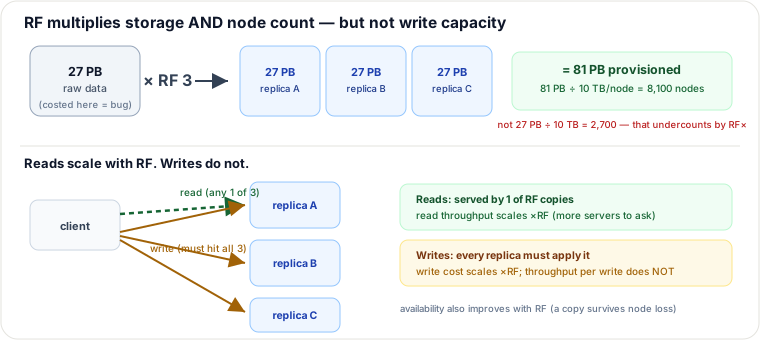
A replication factor (RF) means every byte written physically exists in RF copies. That single fact multiplies storage (RF copies of the same data), node count (RF copies need RF× the machines), and write cost (every copy must independently apply the write) — and it multiplies read capacity too, because any one of the RF copies can answer a read. Size an estimate off the raw dataset and you under-provision storage, nodes, and write throughput all at once by exactly RF×, while crediting yourself with read headroom you were never actually short on.

The storage trace: 27 PB raw → 81 PB provisioned

Take the photo-service estimate from the storage estimation playbook: 10M photos/day at ~1.5 MB each, kept 5 years, comes to ~27 PB of raw data before replication.

Step	Arithmetic	Result
Raw data	given	27 PB
Provisioned storage	27 PB × RF 3	81 PB
Usable capacity per node	given	10 TB
Nodes needed (correct)	81,000 TB ÷ 10 TB	8,100 nodes
Nodes needed (bug: sized off raw)	27,000 TB ÷ 10 TB	2,700 nodes — 3× too few

Whoever costs the "27 PB" line item and racks 2,700 nodes has quietly under-provisioned by exactly RF×. The storage bill, the rack count, and the network fabric all have to be sized off 81 PB, not 27.

Single-node fit is a shard question, not a whole-dataset question

"Does this fit on one node?" is never asked about the full 81 PB — it's asked about the shard (partition) that a single node owns. Once the data is sharded across the 8,100 nodes above, each node holds roughly its 10 TB slice, and the fit question (is this shard's working set too big for RAM/SSD, is this shard too hot) is local to that slice. It has nothing to do with how many total nodes RF forced you to buy — but the two mistakes compound: get RF wrong and the node-count denominator is wrong, which makes "data ÷ nodes = shard size" wrong too, even if you correctly think about fit per-shard.

Reads scale with RF. Writes do not.

Mechanism: a read can be answered by any single replica — a load balancer (or, under quorum, whichever R replicas are contacted) picks from RF available copies, so RF replicas running in parallel serve up to RF× the read QPS one copy could alone. A write is different: it isn't durable until it has been applied to (a quorum of) the copies, so every write generates RF units of write work — one apply per replica — regardless of how many replicas exist. Adding replicas buys read throughput and availability (lose one node, RF−1 copies still answer) at the direct, unavoidable cost of RF× the write-side work and RF× the storage.

The quorum tie-in

RF is also what sets N in the quorum equation — N = RF, and you pick R and W so that R + W > N for strong consistency (see quorum). RF = 3 with R = 2, W = 2 is the classic Dynamo-style default: R + W = 4 > 3, and every read set and write set is guaranteed to overlap on at least one up-to-date replica. Raising RF gives more slack in choosing R and W (e.g. R = 1 for faster reads while W stays high) — but every extra replica added to N adds to the same storage and write-cost multiplier derived above.

Pitfalls

• Costing the raw number. Racking or budgeting for 27 PB instead of 81 PB under-provisions storage and nodes by RF× at once — the single most common capacity-estimation bug.
• Assuming RF helps writes. RF helps reads and availability; it does nothing for write throughput and actively costs write capacity — RF× the applies, RF× the network fan-out, per write.
• Conflating whole-dataset fit with shard fit. "Does it fit on one node" is answered per-shard (data ÷ node count), never against the full 81 PB — and an RF mistake upstream silently breaks this answer too, since it changes the node-count denominator.

Judgment: RF = 3, higher RF, or erasure coding?

RF = 3 is the default (Dynamo, Cassandra, HDFS, Kafka) because it's the smallest N where a quorum (R + W > N) tolerates one node failure while each of R and W still needs only a proper subset of N (not all replicas) — solid durability and availability for a 3× storage/write tax.

Higher RF (4, 5) survives more simultaneous failures and gives more read fan-out headroom, at a linear extra cost in storage and write work — used for small, hot, must-not-lose data (metadata/config services), rarely for bulk data because the storage tax scales linearly with RF.

Erasure coding is the named alternative: instead of RF whole copies, split data into k data shards + m parity shards across k+m nodes (e.g. 6-of-9, as HDFS-EC and Facebook's f4 blob store do) and reconstruct any k from any surviving k+m − losses. Storage overhead drops from RF× (3× = 200% overhead) to roughly (k+m)/k (6+3 → 1.5× = 50% overhead) — a large storage win over RF = 3. The cost: reconstructing a lost shard or serving a read after a failure means decoding across k shards (real CPU and network), and every write must fan out to k+m shards with parity computed, so it fits cold/warm, rarely-rewritten data (archival, blob storage) far better than hot, small, latency-sensitive records where RF's O(1) read/rebuild wins.

Takeaways

• RF multiplies three things at once: storage (RF×), node count (RF×), and write cost (RF×) — costing the raw dataset size under-provisions all three by exactly RF.
• Reads scale with RF (any 1-of-RF replica can answer); writes do not (every replica must apply every write).
• Single-node fit is a per-shard question (data ÷ node count), never a whole-dataset question — and RF sets that denominator.
• RF = 3 is the durability/availability default and sets your quorum's N; erasure coding trades CPU/rebuild cost for a much lower storage multiplier when data is cold enough to afford the decode cost.

---

Storage arithmetic continues the photo-service example from this guide's storage-estimation playbook. Replication/quorum mechanics per Amazon's Dynamo paper (DeCandia et al., 2007) and the Apache Cassandra replication docs; erasure-coding trade-offs per Apache Hadoop's HDFS Erasure Coding design and Facebook's f4 warm blob storage (Muralidhar et al., OSDI 2014). Re-authored and traced for this guide.

I just read a lesson on **Replication in Capacity Estimation** (System Design) and want to truly understand it. Explain Replication in Capacity Estimation from first principles using ONE vivid real-world analogy and a visual mental model — draw it as ASCII art or a clear step-by-step diagram — with a concrete example using real numbers. Then ask me one question to check I got the mental picture, and wait for my reply. If you're unsure or a claim isn't standard, say so and reason from first principles instead of guessing.

Teach me **Replication in Capacity Estimation** interactively. Ask me ONE guiding question at a time, wait for my answer, and adapt to my confusion — build the idea with me step by step instead of explaining it all at once. If you're unsure or a claim isn't standard, say so and reason from first principles instead of guessing.

Quiz me on **Replication in Capacity Estimation** with 5 questions, easy to tricky, ONE at a time. Tell me if each answer is right; at the end, explain clearly what I got wrong and why. If you're unsure or a claim isn't standard, say so and reason from first principles instead of guessing.

Help me remember **Replication in Capacity Estimation** for the long term: give the one-sentence intuition, a memorable hook/mnemonic, a tiny worked example, and 3 active-recall flashcards (Q -> A). If you're unsure or a claim isn't standard, say so and reason from first principles instead of guessing.