Capacity Estimation — The Senior Corrections: Fan-out, Peak Factor, 70% Utilization & Durability (Deep Dive)
The gates you memorized are compressed derivations — decompress them
The estimation playbook teaches “fan-out ~20–50×”, “peak ~2–10×”, “target ~70% utilization”, “replicate 3×” as facts to recall under interview pressure. Each one is really the compressed output of a short derivation, and a senior candidate is expected to re-expand the compression on demand — not just quote the number, but say why this workload lands at 50× and not 20×, why this traffic pattern gives 2.4× and not 10×, why 70% and not 90%. This page walks the four gates from the estimation unit (fan-out, peak factor, utilization, durability) and adds exactly that layer: the arithmetic that turns “I remember the number” into “I can derive the number for a workload I have never seen.” Where this guide already has a full derivation of a piece (tail-latency fan-out, the M/M/1 curve, replication-factor durability, retry storms), this page recomputes the headline numbers compactly and points to the deep page for the full proof — the goal here is the connective judgment layer across all four gates at once, not a fifth restatement of any one of them.
1. Fan-out: a feed read is not one backend query
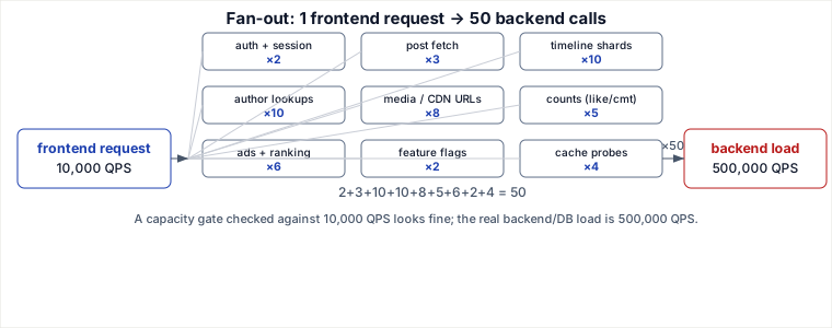
Mechanism: a single frontend request is answered by calling many internal services, and every one of those calls is itself a request the backend fleet must serve — so downstream QPS = frontend QPS × fan-out factor, and the fan-out factor is a sum over every service the request actually touches, not a guess.
Traced: 10,000 req/s at the edge, 500,000 req/s at the backend
Take a social-feed read. Nothing about “load the feed” is answered by one query — opening it triggers auth, the post fetch, per-shard timeline assembly, author lookups for each post, media URL signing, social counts, ads/ranking, feature-flag checks, and cache probes:
| Call group | Calls per request |
|---|---|
| Auth + session check | 2 |
| Primary post fetch | 3 |
| Timeline assembly across shards | 10 |
| Author/profile lookups (per post) | 10 |
| Media / CDN URL signing | 8 |
| Social counts (likes/comments/shares) | 5 |
| Ads + ranking calls | 6 |
| Feature-flag / experiment lookups | 2 |
| Cache-tier probes (L1+L2) | 4 |
| Total fan-out factor | 50 |
Backend QPS = 10,000 × 50 = 500,000 req/s. That is the number a capacity gate must be checked against — not the 10,000 the load balancer reports. This is the correction that matters before declaring “no exotic architecture needed”: a common playbook gate says a single primary comfortably takes ~3,000–5,000 writes/s. Checked against 10,000 frontend QPS, that gate looks generous. Checked against the real 500,000 backend QPS it implies, you are 100–500× over a single node and sharding is not optional. Apply the fan-out correction before comparing anything to a per-node ceiling, or the comparison is meaningless.
The same fan-out also amplifies the tail, not just the volume
A wide fan-out has a second, independent cost: if every one of the 50 (here, up to N≈100 in a heavier case) backend calls is fast 99% of the time, the probability all of them are fast on a given request is 0.99100 ≈ 37% — so 63% of requests hit at least one slow sub-call, and the parent request’s typical latency becomes its slowest dependency’s p99, not its average. This tail-fan-out derivation (P(all fast) = P_fastN) is proved in full, with the hedged-request and timeout defenses, on the tail-latency & fan-out and the systems-cheat-sheet pages — the point to carry here is that the QPS correction above and the latency correction are the same fan-out, hitting two different budgets (throughput and SLO) at once.
2. Peak factor from first principles: why ~2–3×, not 10×
Mechanism: average QPS = requests/day ÷ 86,400s assumes traffic is spread evenly across every second of the day. Real traffic is not uniform — it concentrates into waking hours plus an evening spike — and the peak multiplier is exactly the ratio between how concentrated the traffic actually is and how concentrated it would be if it were flat.
The rounding trap most estimators never quantify
Before the peak factor, one constant is worth being precise about. 600,000,000 requests/day ÷ 86,400 s = 6,944.4 req/s, exactly. Round the divisor to 105 (100,000) for mental math and you get 600,000,000 ÷ 100,000 = 6,000 req/s instead — a shortfall of 944.4, i.e. (6,944.4 − 6,000) / 6,944.4 ≈ 13.6%. That is fine for a first-pass BOTE (round in the direction that keeps you conservative, and say so out loud), but it is worth knowing the rounding itself quietly removes ~14% of the true QPS before any peak factor is even applied — stacking a peak multiplier onto an already-undercounted average compounds the error in the wrong direction if you are sizing a hard ceiling rather than a rough plan.
Deriving ~2–3× for a single-timezone consumer pattern
The general rule — peak factor = (share of traffic in a window) ÷ (share of the day that window occupies) — is derived in full on the peak-factor-derivation page, including the compounding “burst inside the busy window” layer that produces the higher end of “2–10×” folklore. The piece worth tracing separately is why a single-timezone consumer social product specifically lands at the low end (~2–3×), not the high end:
| Window | Traffic share | Time share | Concentration |
|---|---|---|---|
| Waking + evening hours (8h of 24h) | 70% | 8/24 = 33.3% | 0.70 ÷ 0.333 ≈ 2.1× |
| Evening spike (2h of 24h) | 25% | 2/24 = 8.3% | 0.25 ÷ 0.083 ≈ 3.0× |
A population confined to one timezone cannot spread its waking hours any wider than roughly a 16–18-hour day, and a normal (non-viral) usage curve inside that window rarely concentrates past “most of it in 8 hours, a chunk of that in a 2-hour spike” — which is exactly the 2–3× folklore range, derived rather than assumed. Contrast a genuinely global, multi-timezone product: each region still shows its own ~2–3× regional peak, but the regions’ peaks land at different wall-clock instants (evening in one region overlaps midday in another), so the aggregate, summed-across-regions curve is flatter than any single region’s curve — a global roll-up can show a lower peak factor than a single-timezone product of the same per-user shape, purely because the concentration does not stack. The 10×-and-up range is a different regime entirely: it requires an extra multiplicative burst layer on top of the diurnal one — a flash sale, a viral post, a synchronized cron/push — and that layer has to be derived from the event, not folded into a baseline “peak QPS” constant.
3. The 70% utilization rule, derived from M/M/1
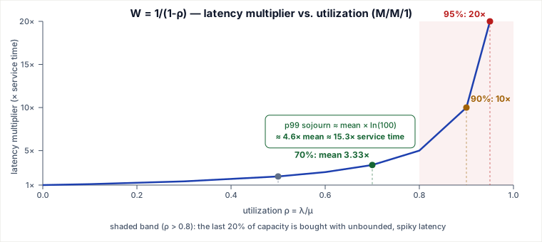
Mechanism: in an M/M/1 queue with utilization ρ = λ/μ, the mean time in system is W = (1/μ) / (1 − ρ) — service time divided by (1−ρ). As ρ → 1 the denominator → 0 and latency blows up hyperbolically, not linearly, which is why “70%” is a derived knee, not a folk number.
| ρ (utilization) | 1 − ρ | W = 1/(1−ρ) × service time |
|---|---|---|
| 0.50 | 0.50 | 2× |
| 0.70 | 0.30 | 3.33× |
| 0.80 | 0.20 | 5× |
| 0.90 | 0.10 | 10× |
| 0.95 | 0.05 | 20× |
Going from 70% to 90% utilization — 20 more points of “capacity used” — triples latency (3.33× → 10×); the next 5 points (90%→95%) double it again. 70% sits just past the point where the curve is still climbing gently; every point past it is bought back at a steeply worse rate. The full derivation, the M/M/1 vs M/M/c pooling argument, and the deterministic-service (M/D/1) comparison live on the Little’s Law & utilization page — the two corrections below are what that page does not cover.
Correction A: 70% bounds the mean. p99 needs its own multiplier
W above is a mean. For M/M/1 specifically, the total sojourn time of a random arrival is itself exactly exponentially distributed with rate (μ−λ) — a standard, exact queueing-theory result, not an approximation — so its own p99 is a fixed multiple of its mean: p99 ≈ W × ln(100) ≈ 4.6 × W, regardless of ρ. At ρ=0.7, mean W is 3.33× service time, so p99 ≈ 3.33 × 4.6 ≈ 15.3× service time — not 3.33×. The 70%-knee argument bounds the average user’s latency; the p99 SLO a senior actually gets paged on needs headroom on top of the knee, not just below it.
Correction B: the target must survive losing a box
70% aggregate utilization across a fleet of N boxes assumes all N are up. Lose one during a deploy or failover and the same λ lands on N−1 servers: ρ′ = ρ × N/(N−1). The erosion is brutal on small fleets:
| Fleet size N | ρ after losing 1 box (from 70% baseline) | Baseline needed to stay ≤70% after losing 1 |
|---|---|---|
| 20 | 0.70 × 20/19 ≈ 0.737 | 0.70 × 19/20 = 0.665 |
| 10 | 0.70 × 10/9 ≈ 0.778 | 0.70 × 9/10 = 0.63 |
| 5 | 0.70 × 5/4 = 0.875 | 0.70 × 4/5 = 0.56 |
| 3 | 0.70 × 3/2 = 1.05 (unstable) | 0.70 × 2/3 ≈ 0.467 |
A 3-box fleet running its “safe” 70% baseline is already past ρ=1 — queue growing without bound — the moment it loses one box, even at perfectly average load, no peak involved. The smaller the fleet, the lower the real target has to be; “70%” is a fleet-size-dependent number, not a universal constant, and this is exactly why N+1 sizing exists as a separate discipline from utilization targeting.
4. Durability / replica-count reasoning
Mechanism: a replica survives independently of its siblings, so the chance of losing every copy of a block falls exponentially with replica count — but the number that actually decides “3” is the never-zero-spare-copies-during-repair argument, not the raw exponential.
The full derivation is on the DFS durability page: with a per-disk annual failure rate p≈2%, the naive independence model gives RF=3 about 5 nines of annual durability (p3 = 8×10⁻⁶); folding in a realistic repair window (the gap between a failure being detected and the block being re-replicated) tightens that to roughly 10.6 nines — because RF=3 is really “never let a repairing block sit at zero spare copies,” and 2 copies is exactly the minimum that survives one loss while a third is rebuilt. That page also derives the erasure-coding trade-off: Reed-Solomon coding buys comparable or better durability at roughly 1.5× storage overhead versus RF=3’s 3× (200% overhead) — the right call for cold data, because EC pays it back on every read/repair with a reconstruction cost RF never has. The storage/write/read multiplication that RF drives (81 PB provisioned from 27 PB raw; reads scale with RF, writes do not) is traced on the replication-in-capacity-estimation page.
Durability and availability are two different axes, and RF conflates them
Replication factor is usually justified as durability, but the copies that give you durability are also, incidentally, what give you failover: a primary-only system with zero extra replicas has no standby to promote when the primary dies, regardless of how durable the underlying storage is (imagine data that is durably fsynced to a network-attached durable log or object store — that alone gives durability with RF=1, but the service still goes down until a new primary reads that log back in). HA needs ≥1 additional replica for failover as a requirement separate from durability’s replica count — real systems often use the same replicas for both, which is efficient, but a senior should be able to say which requirement is driving the number when they diverge (e.g., durability alone might tolerate RF=2 with a fast durable backup, but failover without a user-visible blip still wants a warm standby).
Capacity-fits ≠ load-fits: what a hot key does to its own replica set
RF=3 gives any one key exactly 3 nodes that can serve it, no matter how many thousand other nodes sit in the cluster. An average key at, say, 10 QPS is trivial for 3 replicas (30 QPS of read capacity against 10 QPS of demand — huge margin). A viral/hot key at 500× that — 5,000 QPS — still only has those same 3 replicas to answer it: ≈1,667 QPS per replica for one key, and if that key needs coordinated writes (a counter increment, a single-writer lock), the ceiling per node for that one key is often set by coordination overhead, not raw throughput, and can sit well below what the node’s aggregate hardware could otherwise do. The cluster’s aggregate capacity budget can be enormous and still irrelevant — the hot key is bottlenecked on the 3 machines that happen to hold it, not on the cluster.
Pitfalls that break plug-in-the-formula readers
- Retry-storm multiplier. A degrading dependency does not add load linearly — effective load = arrivals ÷ (1−p) as retry-probability p climbs, and at p=2/3 a 10,000 req/s baseline becomes 30,000 req/s at the same struggling store, a positive feedback loop that outlives its trigger. Fully traced, with the GC-pause worked example, on the fan-out & retry-storms page and the load-balancing sizing page (the 3-tier 3×3×3=27× compounding case). Do not size a dependency’s capacity off its calm-state QPS.
- Cache stampede / thundering herd + hot-key-on-one-shard. A key expiring at a single instant makes every concurrent reader miss at once and hammer the origin simultaneously; a hot key concentrates that same load onto whichever one shard happens to own it, independent of overall cluster headroom — the mechanism (XFetch probabilistic early refresh, single-flight, salting) is on the caching-stampede and cache-stampede pages. Capacity-fits ≠ load-fits (above) is the same failure mode viewed from the durability side.
- The “hot fraction” is not a constant. “Cache the hot 20%” describes one observed access-pattern shape (a Zipfian reuse-distance distribution), not a law. The real object is a curve — hit ratio vs. cache size — and the “20%” is just where that curve happens to flatten for that workload: a Zipfian pattern might give ~60% hit ratio at 10% cache size, ~80% at 20%, ~90% at 40%, ~97% at 80% (steep knee, matches the 80/20 folklore); a uniform-random access pattern gives a straight line, hit ratio ≈ cache fraction, with no knee and no “hot fraction” at all. Measure the curve for your own access log before sizing off “20%.”
- Storage is a ceiling only if writes are flat and nothing is deleted. The standard formula (writes/day × bytes × retention × RF) assumes a flat write rate. At a steady 15 TB/day for 5 years that is ~27 PB raw; growing writes 20%/year compounding instead gives ∑ (y=0..4) 1.2y × 15 TB × 365 ≈ 7.44 × 5,475 TB ≈ 40.7 PB — about 49% more than the flat estimate, from growth alone. Symmetrically, if deletes/TTL expiry offset a large share of writes, “total ever written” wildly overstates steady-state storage — the ceiling assumption breaks in both directions, and either one silently invalidates a number that looked done.
- Origin-vs-edge bandwidth decomposition. A CDN gate like “500 Gbps of egress” (100K concurrent HD streams × 5 Mbps, from the bandwidth playbook) is the edge’s number, not the origin’s. Origin bandwidth = total bandwidth × (1 − hit ratio): at a 95% CDN hit ratio, the origin only has to sustain 500 Gbps × 0.05 = 25 Gbps (≈3.1 GB/s) — but that 5% miss/fill path is exactly the path the CDN tail-latency page shows dominates p99, so it is also the path that must be provisioned, not waved away as “the CDN handles it.”
- Back-pressure / safe queue depth. A bounded queue still needs its bound sized, and Little’s Law gives it directly: safe_depth ≈ λ × acceptable_wait. At 5,000 req/s arrivals and a 200 ms acceptable p99 wait, safe_depth ≈ 5,000 × 0.2 = 1,000 items — beyond that, shed (429/503) rather than keep enqueuing; the three-way block/drop/degrade choice is on the back-pressure-mechanisms page.
Judgment layer
When 2–3× peak is enough vs. when it is not: bake the derived diurnal factor (2–3× for a normal single-timezone consumer curve) into standing baseline capacity — it is predictable and repeats daily. Reach for a higher factor, and treat it as a separate autoscale/shed layer rather than a bigger baseline constant, whenever the traffic has an event driver on top of the diurnal shape: a launch, a marketing push, a viral post, a synchronized client-side cron/push. Those compound multiplicatively with the diurnal factor (2.4× × 5× ≈ 12× in the peak-factor-derivation page’s worked event), and no fixed “peak = average × k” constant survives contact with an actual flash crowd — derive the ratio from the event’s own shape (traffic share ÷ time share) instead.
When “3K writes/s is fine” is NOT fine: that gate is a per-node/per-shard ceiling, checked against a per-node/per-shard number — it silently stops being fine the moment either (a) fan-out has not yet been applied, so the number being checked is the frontend QPS instead of the real backend QPS landing on that tier, or (b) load is not uniform across shards, so one shard (holding a hot key, an unlucky hash range, or a popular account) carries far more than the cluster average even while the fleet-wide mean sits comfortably under budget. Always ask “3K/s of what traffic, checked against which shard” before accepting the gate.
Takeaways
- Every BOTE gate here (fan-out, peak factor, 70% utilization, RF=3) is a compressed derivation. Know the derivation, not just the constant, so you can tell a senior interviewer why your workload lands where it does — and recognize when it lands somewhere else.
- The gates compound multiplicatively, not independently: fan-out × peak × hot-key concentration can turn a comfortable-looking average into an overloaded shard even when every individual gate was checked and passed.
- Averages hide the two things that actually cause outages: concentration (a hot key/shard, a burst window, a p99 tail) and feedback (retries, cascading fan-out, a queue that never drains). A number with no concentration/feedback check behind it is not yet an estimate.
- “70%”, “RF=3”, “2–3× peak” are correct defaults for a plain, single-timezone, steady-write, uniformly-loaded system — and every one of those five qualifiers is a place the default can silently stop applying.
The transfer twist
A plug-in-the-formula reader is handed: frontend averages 2,000 QPS, fan-out is 50×, peak factor is 3×, spread evenly across 20 shards. They compute 2,000 × 50 × 3 = 300,000 QPS, divide by 20 shards = 15,000 QPS/shard, check it against the per-shard gate, and call the design done. The number the formula never surfaces: one celebrity account’s data draws 2% of all reads, and it lives on exactly one of those 20 shards. That shard’s load is not its even 1/20th share — it is (98% of 300,000 spread over 20 shards ≈ 14,700) plus the full 2% × 300,000 = 6,000 concentrated onto it alone ≈ 20,700 QPS, roughly 41% over every other shard’s ~14,700. The aggregate math was exactly right and the design still falls over on one shard, because fan-out, peak, and hot-key concentration were each checked in isolation instead of stacked on the one place they all land at once.
Related pages
- Deriving the Peak Factor (not memorizing x2-10) — the full derivation of the peak-factor gate this page recomputes compactly.
- Queueing Non-Linearity — Little’s Law & Utilization — the full M/M/1, M/M/c pooling, and M/D/1 derivation behind the 70% knee.
- Distributed File System — Durability Arithmetic, Erasure Coding, Hot Blocks & NameNode Split-Brain (Deep Dive) — the full RF=3 vs erasure-coding durability arithmetic this page’s section 4 summarizes.
- Traffic Amplification: Fan-out & Retry Storms — the retry-storm feedback-loop mechanism referenced in the pitfalls section.
- Replication in Capacity Estimation — how RF drives storage, write, and read multiplication in a capacity budget.
Derivations synthesized from standard M/M/1 queueing theory (Kleinrock), the exact M/M/1 sojourn-time distribution (Exponential(μ−λ)), Dean & Barroso's “The Tail at Scale” (CACM 2013), Backblaze annual drive-reliability statistics (durability), and this guide's own peak-factor-derivation, queueing-Little's-Law-utilization, traffic-amplification, and DFS-durability pages, cross-referenced rather than restated. Re-authored/Deepened for this guide.
🤖 Don't fully get this? Learn it with Claude
Stuck on Capacity Estimation — The Senior Corrections: Fan-out, Peak Factor, 70% Utilization & Durability (Deep Dive)? Open Claude, copy a block below, and it'll teach you this exact concept — visually and interactively.
Build the mental picture, not memorization.
I just read a lesson on **Capacity Estimation — The Senior Corrections: Fan-out, Peak Factor, 70% Utilization & Durability (Deep Dive)** (System Design) and want to truly understand it. Explain Capacity Estimation — The Senior Corrections: Fan-out, Peak Factor, 70% Utilization & Durability (Deep Dive) from first principles using ONE vivid real-world analogy and a visual mental model — draw it as ASCII art or a clear step-by-step diagram — with a concrete example using real numbers. Then ask me one question to check I got the mental picture, and wait for my reply. If you're unsure or a claim isn't standard, say so and reason from first principles instead of guessing.
Socratic — adapts to where you're stuck.
Teach me **Capacity Estimation — The Senior Corrections: Fan-out, Peak Factor, 70% Utilization & Durability (Deep Dive)** interactively. Ask me ONE guiding question at a time, wait for my answer, and adapt to my confusion — build the idea with me step by step instead of explaining it all at once. If you're unsure or a claim isn't standard, say so and reason from first principles instead of guessing.
Active recall exposes what you missed.
Quiz me on **Capacity Estimation — The Senior Corrections: Fan-out, Peak Factor, 70% Utilization & Durability (Deep Dive)** with 5 questions, easy to tricky, ONE at a time. Tell me if each answer is right; at the end, explain clearly what I got wrong and why. If you're unsure or a claim isn't standard, say so and reason from first principles instead of guessing.
Intuition + hook + flashcards for long-term memory.
Help me remember **Capacity Estimation — The Senior Corrections: Fan-out, Peak Factor, 70% Utilization & Durability (Deep Dive)** for the long term: give the one-sentence intuition, a memorable hook/mnemonic, a tiny worked example, and 3 active-recall flashcards (Q -> A). If you're unsure or a claim isn't standard, say so and reason from first principles instead of guessing.