hard Queueing Non-Linearity — Little's Law & Utilization
Little’s Law is a relationship, not a capacity ceiling
L = λW says the average number of items in a system (L) equals the arrival rate (λ) times the average time each spends in the system (W). It is a conservation law — true for any stable system regardless of arrival or service distribution — but on its own it says nothing about how latency behaves as load rises: it relates three averages, it does not predict them. The engineering danger is reading “the server handles 1000 rps” as a flat wall you can safely push right up to. It is not. To see what actually happens to latency, you need a queueing model.
The M/M/1 result that changes how you provision
Model one server with Poisson arrivals at rate λ and exponential service at rate μ (mean service time 1/μ). Define utilization ρ = λ/μ (the fraction of time the server is busy; it must be < 1 or the queue grows without bound). The standard results are:
L = ρ / (1 − ρ)        (mean number in system)
W = 1 / (μ − λ) = (1/μ) / (1 − ρ)   (mean time in system)
Read that second formula: W is the raw service time divided by (1 − ρ). As ρ → 1 the denominator → 0 and W blows up hyperbolically — not linearly. Doubling load from 40% to 80% does not double latency; it can multiply it many times over.
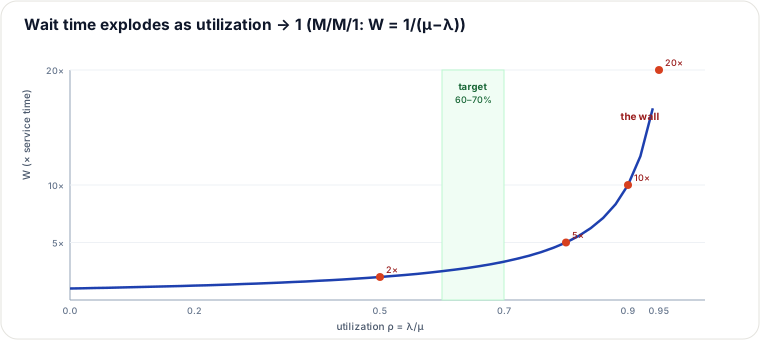
Worked table: the last 30% of capacity costs the most latency
Take service time as 1 unit (1/μ = 1), so W is measured in multiples of the raw service time.
| ρ (utilization) | 1 − ρ | W = 1/(μ−λ) | L = ρ/(1−ρ) |
|---|---|---|---|
| 0.50 | 0.50 | 2× | 1 |
| 0.70 | 0.30 | 3.33× | 2.33 |
| 0.80 | 0.20 | 5× | 4 |
| 0.90 | 0.10 | 10× | 9 |
| 0.95 | 0.05 | 20× | 19 |
| 0.99 | 0.01 | 100× | 99 |
Going from 50% to 90% utilization added 40 points of “capacity used” but multiplied latency 5× (2× → 10×). The jump from 90% to 95% — just 5 more points — doubles it again (10× → 20×). That is why the operational target is roughly 60–70% utilization: below the knee of the curve latency is stable and predictable; the last slice of capacity is real throughput on paper but is paid for in unbounded, spiky latency.
And M/M/1 is optimistic: it assumes smooth Poisson arrivals. Real traffic is burstier, and higher variance makes the queue worse at the same ρ — another reason to keep headroom.
Pitfalls
- Confusing throughput with latency. A system can be “handling” 95% load and hitting SLA on throughput while p99 latency has already fallen off the cliff.
- Provisioning to average, not to peak. If average ρ is 0.7 but a daily peak hits 0.95, your peak latency is 20×, not 3.33×. Size to peak ρ.
- W (time in system) vs Wq (time waiting in queue). W = Wq + service time; the queue-wait portion is what explodes. Don’t compare the wrong one to your SLA.
- Pushing ρ ≥ 1 momentarily (a lost server, a traffic spike) sends the queue → ∞ and the system into congestion collapse — recovery needs load-shedding, not just waiting.
The judgment layer
Headroom vs cost. Targeting 60–70% deliberately “wastes” 30–40% of hardware. What you buy with it is bounded, predictable tail latency plus slack to absorb bursts and to survive losing a server without tipping past ρ=1. Running hot (90%+) saves machines but makes latency fragile: a small traffic bump or one failed node pushes you over the knee and latency explodes. The decision is explicit — how much are you willing to pay in idle capacity to keep p99 flat? — and for latency-sensitive services the answer is “a lot.”
Named alternatives to just buying headroom. More servers sharing one queue (M/M/c) beats the same total utilization split across many single-server queues: a shared queue never leaves one server idle while another has a backlog, so a pool of c servers at utilization ρ has dramatically lower wait than c separate M/M/1 queues each at ρ — this is the economy-of-scale argument for consolidating behind one load balancer. Reducing service-time variance helps too: deterministic service (M/D/1) has half the queueing delay of M/M/1 at the same ρ, so making work uniform (batching, capping request size) flattens the curve. Back-pressure and load-shedding are the last resort — when ρ would exceed the safe zone, reject or defer work to keep ρ < 1 rather than let the queue run away.
Takeaways
- L = λW is an identity about averages; it does not tell you latency-vs-load — add a queueing model for that.
- M/M/1: W = 1/(μ−λ) = service_time/(1−ρ), so latency rises hyperbolically as ρ → 1 (2× at 0.5, 10× at 0.9, 20× at 0.95).
- Target ~60–70% utilization: the last 30% of capacity is bought with unbounded latency and leaves no burst headroom.
- Prefer pooling (M/M/c) and lower variance over running a single server hot; use back-pressure to keep ρ < 1.
Synthesized from Little’s Law (Little 1961), standard M/M/1 / M/M/c queueing theory (Kleinrock), and its operational use in Gunther’s Guerrilla Capacity Planning and the Google SRE workbook (utilization vs latency). Re-authored/Deepened for this guide.
🤖 Don't fully get this? Learn it with Claude
Stuck on Queueing Non-Linearity — Little's Law & Utilization? Open Claude, copy a block below, and it'll teach you this exact concept — visually and interactively.
Build the mental picture, not memorization.
I just read a lesson on **Queueing Non-Linearity — Little's Law & Utilization** (System Design) and want to truly understand it. Explain Queueing Non-Linearity — Little's Law & Utilization from first principles using ONE vivid real-world analogy and a visual mental model — draw it as ASCII art or a clear step-by-step diagram — with a concrete example using real numbers. Then ask me one question to check I got the mental picture, and wait for my reply. If you're unsure or a claim isn't standard, say so and reason from first principles instead of guessing.
Socratic — adapts to where you're stuck.
Teach me **Queueing Non-Linearity — Little's Law & Utilization** interactively. Ask me ONE guiding question at a time, wait for my answer, and adapt to my confusion — build the idea with me step by step instead of explaining it all at once. If you're unsure or a claim isn't standard, say so and reason from first principles instead of guessing.
Active recall exposes what you missed.
Quiz me on **Queueing Non-Linearity — Little's Law & Utilization** with 5 questions, easy to tricky, ONE at a time. Tell me if each answer is right; at the end, explain clearly what I got wrong and why. If you're unsure or a claim isn't standard, say so and reason from first principles instead of guessing.
Intuition + hook + flashcards for long-term memory.
Help me remember **Queueing Non-Linearity — Little's Law & Utilization** for the long term: give the one-sentence intuition, a memorable hook/mnemonic, a tiny worked example, and 3 active-recall flashcards (Q -> A). If you're unsure or a claim isn't standard, say so and reason from first principles instead of guessing.