What is Little’s Law and How to Use It for Quick Capacity Estimates in System Design

Little’s Law is a simple queueing theory formula that states a system’s average number of items in progress equals the average arrival rate multiplied by the average time each item spends in the system.

This fundamental relationship, discovered by John Little in the 1960s, provides a powerful way to analyze queues and performance in both everyday scenarios and computer systems.

In essence, it links three key metrics, including throughput, time, and concurrency, with a surprisingly straightforward equation.

Understanding Little’s Law (Meaning and Formula)

Little’s Law can be expressed algebraically as L = λ × W, where each term represents:

• L (Load or Concurrency): the average number of items in the system simultaneously (e.g. customers in line, or requests “in flight” being processed). This is sometimes called work in progress (WIP) in process terms.

• λ (Throughput or Arrival Rate): the average rate at which items enter and exit the system (e.g. requests per second hitting a server).

• W (Wait Time or Latency): the average time each item spends in the system, from arrival to completion (e.g. the response time per request).

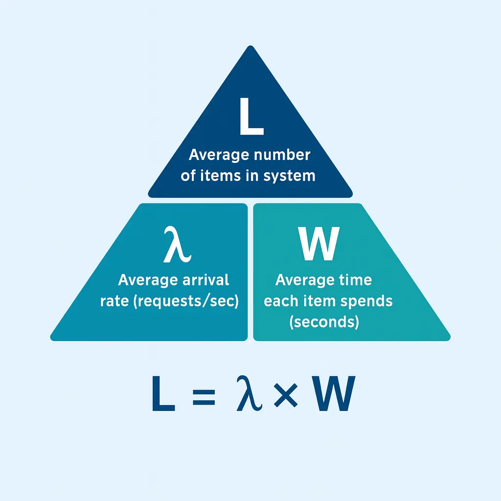
In plain language, Little’s Law says that at steady state, Number of Items in System = Arrival Rate × Time in System.

For example, imagine a coffee shop: if customers arrive at 10 per minute and each spends 0.5 minutes in the shop, there will be about 5 customers on average inside at any time (10 × 0.5 = 5).

If service slows down (customers stay longer), more people will pile up in the store even if arrivals per minute stay the same.

From checkout lines to network requests, this intuitive idea holds for any stable queueing system, regardless of process details, as long as the system is in a steady state (arrivals and completions balanced on average).

One remarkable aspect of Little’s Law is its generality: it does not depend on the distribution of arrivals or service times or the order of service.

This makes it widely applicable. It’s used in manufacturing and agile workflows as well (often phrased as WIP = throughput × cycle time in those contexts).

The formula implies that if you know any two of the three variables (L, λ, W), you can always calculate the third.

This simple relationship is the cornerstone for many capacity planning and performance analysis tasks.

Why Little’s Law Matters in System Design

In system design and performance engineering, Little’s Law is extremely important because it connects throughput, latency, and concurrency; the very metrics we care about when building scalable systems.

It provides a quick reality check and estimation tool for capacity:

• Capacity Planning: Little’s Law helps determine how much load a system can handle. For instance, if a server can process requests with an average latency of W seconds and can handle L requests in parallel (e.g. due to thread limits or CPU cores), then the maximum throughput (λ) is about L/W requests per second. In other words, throughput ≈ concurrency ÷ latency. Example: If a web server allows 500 concurrent connections and each request takes ~0.5 s on average, it can sustain roughly 1000 req/sec (500 / 0.5 = 1000) before queues start building up. This kind of back-of-the-envelope calculation is invaluable when estimating system capacity requirements during design. One of the primary applications of Little’s Law is indeed capacity planning. By estimating arrival rates and desired service times, you can figure out the needed concurrency (or vice versa) to meet performance goals.

• Bottleneck Identification: Little’s Law highlights that if one factor is out of line, it will affect the others. For example, if latency (W) increases while arrival rate stays constant, the number of in-flight requests L will grow, indicating a potential bottleneck. Engineers use this insight to spot when a system is overloaded or when a component is slowing down the workflow. In fact, speed is capacity. Reducing latency directly increases how many requests per second your system can handle. Conversely, if requests take longer to process, the system “feels” congested because more requests accumulate in progress.

• Universal Insight: Because Little’s Law is so general, it applies to many contexts. In web services and distributed systems, L=λW explains the relationship between throughput (QPS), response time, and concurrency. In project management or agile teams, it relates tasks in progress to delivery rate and lead time. This universality means the concept helps engineers and planners speak the same language about performance whether discussing a database, an API, or a Kanban board. It encourages a holistic view: you can’t change one variable (say, increase throughput) without impacting either concurrency or wait time.

Using Little’s Law for Quick Capacity Estimates in System Design

One of the most practical uses of Little’s Law for engineers is making quick capacity estimates during system design or in interviews.

With two known metrics, you can solve for the third to ensure your design will scale:

1. Estimate Required Concurrency (Threads/Connections)

Suppose you expect a peak throughput of 200 requests per second and you aim for an average latency of 0.5 seconds per request.

Little’s Law predicts you’ll have L = 200 × 0.5 = 100 requests in progress on average. That means your system should be designed to handle about 100 concurrent requests (e.g. via sufficient threads, connection pools, or server instances) to achieve this throughput without queuing delays.

If you provision far fewer (say 50 threads), those extra requests will start queuing up, increasing wait time.

This calculation gives a ballpark capacity estimate for sizing your resources.

2. Determine Maximum Throughput with Given Capacity

In many cases, you know your system’s limits and want to find the throughput.

For example, if a database can handle at most 50 concurrent queries and each query takes ~0.1 s on average, the maximum throughput is about λ = 50 / 0.1 = 500 queries per second.

Pushing beyond ~500 QPS will result in a queue because the database cannot process more than 50 at once without slowing down.

Little’s Law thus helps set an upper bound on throughput given fixed capacity and response times.

3. Validate Performance Targets

Little’s Law can also validate if a performance target is realistic.

For instance, if an API service must handle 1,000 req/sec and current average latency is 0.5 s, it implies 500 concurrent requests are in flight on average.

If your architecture only supports 100 concurrency, you either need to drastically cut latency (to ~0.1 s) or increase concurrency (e.g. add servers or threads) to meet the target.

This kind of quick math is often used in system design discussions and interviews to sanity-check proposals.

Example Scenario: Applying Little’s Law to a Web Service

To make this concrete, consider a web API handling user requests.

Imagine it currently processes 200 requests/second and each request takes 0.5 s to complete on average.

By Little’s Law, at any moment about L = 200 × 0.5 = 100 requests are being handled concurrently. Now say a certain operation in the system becomes slower (e.g. a database call starts taking longer), and the average response time increases to 2 s.

If the arrival rate remains 200 req/sec, the equation predicts L = 200 × 2 = 400 concurrent requests in flight.

Without any change in traffic, the system suddenly has 4× more load!

This explosion in concurrent load is why a slowdown in one component (higher latency) makes the whole system feel overloaded.

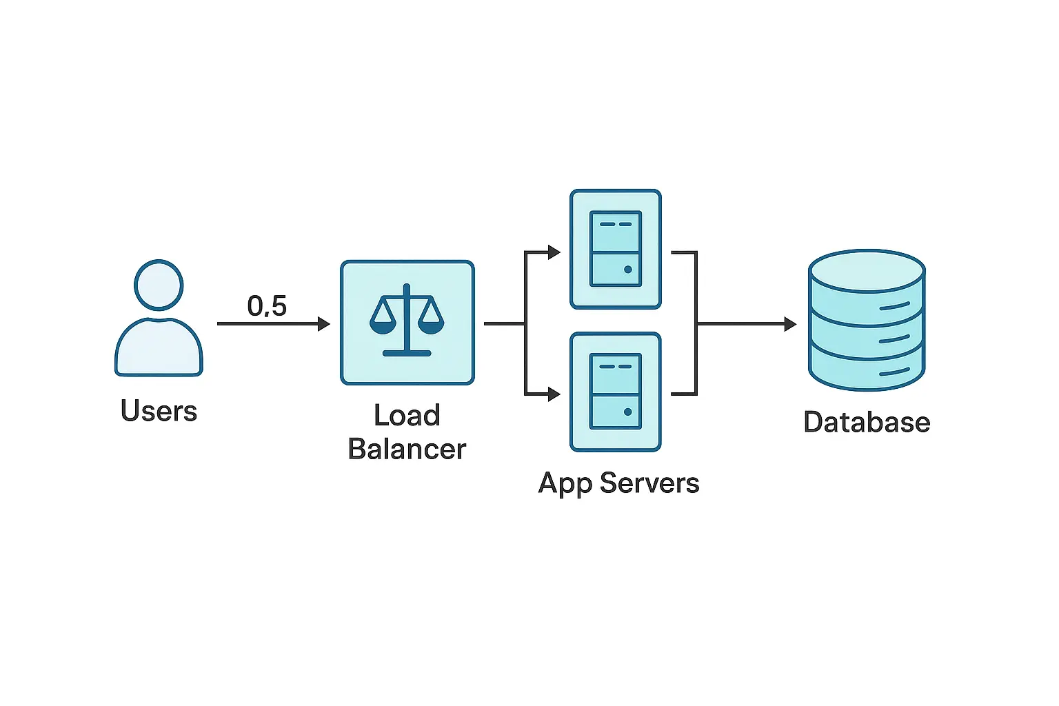
In practice, you would need to add capacity (more threads, instances, or caching) to handle 400 concurrent requests, or work on reducing the latency back down, to stabilize the system.

Little’s Law gives you this intuition and the numbers to quantify it: faster service = fewer in-flight requests, which means higher throughput capacity, whereas slow service causes requests to backlog.

The example also illustrates a key point: simply adding servers isn’t always a silver bullet.

If the 2 s lives in a shared downstream — the slow database call — then adding app servers changes nothing the user feels: W is still 2 s, total in-flight is still λ × W = 400 (now just spread thinner across more idle app servers), and the database remains the queue. Horizontal scaling only raises capacity when the added nodes add capacity at the bottleneck; Little’s Law applied per-tier (measure L, λ, and W for the DB alone) is how you find which tier that is.

The law teaches that you must either reduce the time each request spends or increase the total concurrency available (e.g-. via horizontal scaling or asynchronous processing) to improve throughput.

Often, improving efficiency (lowering W) is the more direct way to boost capacity.

Key Takeaways and Best Practices

• Remember L = λW: Little’s Law is an easy formula but packs a punch. Keep it in mind when designing or debugging systems. If you have any two of {throughput, latency, concurrency}, you can find the third. Use it to do quick “back-of-the-envelope” calculations for system capacity and to cross-check performance metrics.

• Ensure Steady-State Assumption: The law holds when the system is stable (long-term arrivals ≈ departures). It won’t directly apply during transient spikes or if the system is overwhelmed (e.g. if incoming rate exceeds capacity for a long time, queues grow without bound). So use average rates over a sustained period and make sure you’re evaluating a scenario where the system can catch up.

• Latency Improvements = Higher Throughput: Because reducing response time W directly lowers the in-system count L for a given arrival rate, speeding up your code or database calls effectively increases capacity. Optimizing latency (even by a few milliseconds) can let your system handle more users without needing additional hardware. In contrast, poor latency will “fill up” the system quickly with waiting requests.

• Design with Concurrency in Mind: System design often involves choosing thread pool sizes, connection limits, or server counts. Little’s Law gives a quantitative guide for those decisions. For example, if each server instance handles X concurrent requests comfortably, you can estimate how many instances are needed for your target throughput. It also reminds you that if you expect higher traffic, you either need to allow more parallelism (larger L) or achieve faster processing (smaller W) to keep up.

In summary, Little’s Law is a foundational concept for both engineers and managers to gauge capacity and performance quickly.

It provides a bridge between technical metrics (like latency and throughput) and real-world impact (like how many users or tasks can be handled concurrently).

By applying Little’s Law, you can reason about system limits, plan scaling strategies, and communicate clearly about performance using a simple, proven formula.

Whether you’re tuning a web service or streamlining a workflow, this law offers a reliable compass for capacity estimation and efficient design.

The knee the formula hides: why 80% utilization is fine and 95% melts

Little's Law (L = λW) is an exact identity in steady state, but it quietly assumes the system is in steady state — arrivals are being served, not piling up. The moment you push toward saturation, the term it does not model, queueing delay, takes over W. As utilization ρ (the fraction of capacity in use) approaches 1, waiting time does not rise linearly — it blows up roughly like 1/(1−ρ). Going from 80% to 95% utilization is only a 15-point change in load, but 1/(1−ρ) climbs from 5 to 20, a ~4× jump in queueing delay. That is why a system that "felt fine at 80%" falls over at 95% for no obvious reason: W explodes, and by L = λW the in-flight count explodes with it. Leaving headroom is not waste; it is staying on the flat part of that curve.

Averages lie: size for the tail, not the mean

L = λW uses mean latency, but capacity failures happen in the tail. If a service does 1,000 rps with p50 = 20 ms but p99 = 200 ms, the mean-based thread count (1000 × 0.02 = 20) is nowhere near enough — during the slow requests you need closer to 1000 × 0.2 = 200 concurrent slots, or those p99 requests queue and drag the whole system past the knee above. Size thread pools and connection pools against a high-percentile W, not the average, precisely because the average is what hides the requests that hurt.

Using it as a live diagnostic

Because the three quantities are locked together, instrument all three on one dashboard: an in-flight gauge (L), arrival rate (λ), and latency (W). The identity turns them into a cross-check — if L is climbing while λ is flat, W is degrading and something downstream is slowing, even before latency alerts fire. And under genuine overload the steady-state assumption breaks, so confirm you are measuring completions, not just arrivals: when arrivals exceed capacity the queue grows without bound and no single W describes the system. (Quick self-check: L = 400 at λ = 800/s implies mean W = L/λ = 0.5 s.)

I just read a lesson on **What is Little’s Law and How to Use It for Quick Capacity Estimates in System Design** (System Design) and want to truly understand it. Explain What is Little’s Law and How to Use It for Quick Capacity Estimates in System Design from first principles using ONE vivid real-world analogy and a visual mental model — draw it as ASCII art or a clear step-by-step diagram — with a concrete example using real numbers. Then ask me one question to check I got the mental picture, and wait for my reply. If you're unsure or a claim isn't standard, say so and reason from first principles instead of guessing.

Teach me **What is Little’s Law and How to Use It for Quick Capacity Estimates in System Design** interactively. Ask me ONE guiding question at a time, wait for my answer, and adapt to my confusion — build the idea with me step by step instead of explaining it all at once. If you're unsure or a claim isn't standard, say so and reason from first principles instead of guessing.

Quiz me on **What is Little’s Law and How to Use It for Quick Capacity Estimates in System Design** with 5 questions, easy to tricky, ONE at a time. Tell me if each answer is right; at the end, explain clearly what I got wrong and why. If you're unsure or a claim isn't standard, say so and reason from first principles instead of guessing.

Help me remember **What is Little’s Law and How to Use It for Quick Capacity Estimates in System Design** for the long term: give the one-sentence intuition, a memorable hook/mnemonic, a tiny worked example, and 3 active-recall flashcards (Q -> A). If you're unsure or a claim isn't standard, say so and reason from first principles instead of guessing.