Capacity Estimation Drills — Fan-out Writes, URL-Shortener Keyspace, Rate-Limiter Constraints & Failover Load (Deep Dive)

Four named drills, one discipline: derive the number, don't recite the range

Every capacity-estimation drill has one arithmetic step that actually decides the design — and it is usually the step interview answers skip. This page works that step for four named drills: Twitter-style timeline fan-out writes, a URL-shortener's keyspace, a distributed rate limiter's real bottleneck, and a cache-flush/failover load dump. It leans on three general laws already derived elsewhere in this guide — Traffic Amplification (fan-out and retry multipliers), Peak-Factor Derivation (why "×2–10" is measured, not memorized), and Replication in Capacity Estimation (why RF must multiply storage and nodes and write cost) — and applies each to a concrete, named scenario instead of restating the law in the abstract.

Drill 1 — Twitter timeline fan-out: the write-amplification arithmetic

Fan-out-on-write ("push") turns one tweet into one timeline-insert per follower, because each follower's timeline is a separately materialized, separately cached object. The number that justifies choosing push over computing timelines live is simple multiplication, but it is the number that makes or breaks the design:

timeline inserts/s = tweets/s × average followers per author

Worked: 6,000 tweets/s × 200 average followers = 1,200,000 timeline inserts/s. That is the steady-state write load the fan-out tier must sustain — a number with no relationship to the 6,000 tweets/s the product dashboard reports, exactly the "naive frontend number is a lower bound" trap this guide's Traffic Amplification page names for internal RPC fan-out; here the same shape shows up one layer over, in follower fan-out instead of service fan-out.

Traced: steady state vs. derived peak

Quantity	Arithmetic	Result
Average timeline inserts/s	6,000 × 200	1,200,000/s
Peak multiplier (derived, not asserted)	2.4× diurnal × 5× burst (from the Peak-Factor Derivation page's worked trace)	12×
Peak timeline inserts/s	1,200,000 × 12	14,400,000/s
Fan-out nodes needed (avg), at 50,000 writes/s/node	1,200,000 ÷ 50,000	24 nodes
Fan-out nodes needed (peak)	14,400,000 ÷ 50,000	288 nodes

Note what changed: the peak multiplier is not a memorized "×5" — it is imported from the peak-factor derivation already worked out for this guide (a normal diurnal concentration compounded with a burst window), so a reviewer can check where 12× came from instead of taking it on faith. Sizing the fan-out tier off the average (24 nodes) instead of the derived peak (288 nodes) is a 12× under-build that only shows up the first time traffic actually peaks.

The celebrity exception: push stops being cheap exactly where it matters most

The 200-follower average hides the tail. A single account with 100,000,000 followers breaks the "amortize the merge once" argument for push, because push work scales with that one account's follower count, not with how often it posts:

1. One celebrity post under pure fan-out-on-write = 100,000,000 timeline writes, all triggered by a single row-write to the post store.
2. Even at a sustained 50,000 writes/s on the fan-out tier, that one post takes 100,000,000 ÷ 50,000 = 2,000s ≈ 33 minutes to fully propagate — shared with every normal user's fan-out jobs already queued behind it (the same "stale fan-out" traced in this guide's Fan-out-on-Write vs Fan-out-on-Read page).
3. The fix is not a bigger fan-out tier — it is a design fork: exempt accounts above a follower threshold T from push entirely, and let their followers pull/merge that post in at read time instead. Zero fan-out writes for the celebrity; a cheap, cacheable merge cost for each of their readers.

The decision rule that falls out: push for followers(account) < T, pull for followers(account) ≥ T — a hybrid, not a single global strategy, with T tuned from the fan-out tier's write budget (the point where one account's push cost stops being negligible next to the other 23 nodes' worth of normal traffic).

Drill 2 — URL-shortener keyspace: sizing the code length before anything else

The one number a "full sizing" of a URL shortener actually hinges on is the short-code length L, because it is the only part of the design that cannot be changed later without breaking every already-issued link. A base-62 code of length L (0–9, a–z, A–Z) can address 62^L distinct codes, so L must satisfy:

62^L ≥ N, where N = total URLs the system must ever address

Traced: choosing L for 100 billion URLs

L	62L	vs. N = 100,000,000,000	Verdict
6	56,800,235,584 ≈ 5.68e10	5.68e10 < 1.0e11	Insufficient — runs out before 100B
7	3,521,614,606,208 ≈ 3.52e12	3.52e12 ≫ 1.0e11	Sufficient — 2.84% utilized at 100B codes

So L = 7 is the answer, and it is a hard boundary, not a rounding choice: 6 characters physically cannot hold 100 billion distinct codes (they exhaust at ≈56.8B), while 7 characters hold ≈35× headroom over the target. Tie the rule to record count directly: any N above ≈5.68×10¹⁰ forces a jump from 6 to 7 characters — there is no in-between length in base 62.

The bandwidth of the request path (the part "full sizing" usually skips)

Sizing stops at the keyspace far too often. The redirect path has real QPS and bandwidth too:

Quantity	Arithmetic	Result
Writes/day (100B codes over 10 years)	100,000,000,000 ÷ 3,650 days	≈27,397,260/day
Avg write QPS	27,397,260 ÷ 86,400	≈317 QPS
Avg read QPS (100:1 read:write, shorteners are read-heavy)	317 × 100	≈31,710 QPS
Peak read QPS (2.4× diurnal only — no viral-burst layer assumed for routine redirects)	31,710 × 2.4	≈76,100 QPS
Avg redirect bandwidth (≈1,000 B round-trip: short code in, 302 + long URL out)	31,710 × 1,000 B	≈31.7 MB/s
Peak redirect bandwidth	76,100 × 1,000 B	≈76.1 MB/s

Note the peak row uses only the diurnal layer (2.4×) from the Peak-Factor Derivation page, not the full 12× burst-compounded figure used in Drill 1 — stated explicitly as an assumption, because a shortener's redirect traffic is closer to steady consumer browsing than a flash-crowd write event. Asserting a peak multiplier without saying which layers you're including (and why) is exactly the gap this page exists to close.

Storage, and where the replication factor has to show up

Per-record footprint: 7-byte code + ≈100-byte average long URL + ≈50 bytes of metadata (created-at, owner, click-count) ≈ 157 bytes/record.

Raw storage = 100,000,000,000 × 157 B ≈ 15.7 TB
Provisioned storage = 15.7 TB × RF 3 ≈ 47.1 TB

A sizing that quotes "15.7 TB" and stops has under-stated the real infrastructure footprint by 3× — the same RF-consistency bug this guide's Replication in Capacity Estimation page traces for a photo service (27 PB raw → 81 PB provisioned). The fix is procedural, not arithmetic: RF is applied once, at the end, to every number derived from raw record count — storage, nodes, and write cost alike.

Drill 3 — Distributed rate limiter: bytes aren't the constraint, ops/s to one logical store is

A rate limiter shared across a fleet needs a single logical source of truth for each limited key — every gateway node must agree on the same count, or the limit isn't actually enforced fleet-wide. That forces every request through one counter service (typically Redis), which makes the counter both a potential hot-key/SPOF (this guide's Rate-Limit Hot Keys page traces the single-celebrity-key case) and the fleet's real throughput ceiling — not the network.

The constraint is ops/s, not bytes/s

Reuse the fleet baseline already established for this drill elsewhere in the guide: 60,000 RPS across 20 gateway nodes, every request doing one check-and-increment against the counter store.

Bytes/s to the counter ≈ 60,000 × ~100 B/op ≈ 6 MB/s — trivial for any network.
Ops/s to the counter = 60,000 ops/s, sustained, to one logical Redis deployment.

6 MB/s is not a capacity conversation. 60,000 atomic check-and-increment operations per second against a single-threaded-per-core Redis primary is: a plain INCR ceiling on commodity Redis sits somewhere around 100,000–200,000 simple ops/s per core, and the atomic check-then-increment a rate limiter actually needs (a Lua script or equivalent, not a bare INCR) costs materially more per op than a raw increment. At 60,000 ops/s you are already sitting at roughly a third to two-thirds of a single node's realistic ceiling before any headroom for tail latency, failover, or traffic growth — the real limit on this design is that one logical counter's throughput and p99, not the bytes moving in or out of it.

Sliding-window LOG vs. COUNTER — the memory difference is huge at scale

Two ways to track "how many requests has this key made in the last window," and the memory cost is not a rounding difference between them. Take 10,000,000 active rate-limited keys, each limited to 100 requests per 60-second window:

Approach	What's stored per key	Bytes/key (at the limit)	System-wide (10M keys, all saturated)
Sliding-window LOG	one timestamp entry per request, in a sorted set	100 entries × ≈80 B/entry ≈ 8,000 B	10,000,000 × 8,000 B ≈ 80 GB
Sliding-window COUNTER	one integer count + one window-start marker	≈50 B (fixed, independent of request volume)	10,000,000 × 50 B ≈ 500 MB

That is a ≈160× memory difference, and it does not shrink with scale — it is per-request-logged vs. fixed-size, so the gap widens as request volume per key grows. A capacity slice that says "the rate limiter needs about 500 MB of Redis" has silently assumed the counter design; the exact sliding-window log a correctness-focused answer reaches for first costs 160× more memory for the same key population.

Drill 4 — Cache-flush / failover load dump: a high hit ratio is a fragility, not just a saving

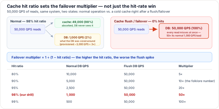
A cache-hit ratio is usually presented as a pure win: 98% of reads never touch the database. But that framing hides the failure mode — the DB was provisioned around the miss traffic, and a cache flush, cold restart, or failover event doesn't reduce the hit ratio gradually. It drops it to 0% instantly, and every one of those reads that used to be absorbed now lands on the database at once.

Failover load multiplier = 1 ÷ (1 − hit ratio)

Traced: the same 50,000 QPS at five hit ratios

Hit ratio	Normal DB QPS	DB QPS right after a full flush	Multiplier
80%	50,000 × 20% = 10,000	50,000	5×
90%	5,000	50,000	10× — the commonly-quoted number
95%	2,500	50,000	20×
98%	1,000	50,000	50×
99%	500	50,000	100×

The "~10× flush spike" folklore is really the 90%-hit-ratio case. Push the same system to 98% — exactly the kind of aggressive cache dependency teams adopt to cut DB cost — and the failover multiplier is 50×, not 10×, because the DB's normal load shrank to almost nothing while the total traffic it must absorb on a flush stayed at the full 50,000 QPS. The better the cache looks day to day, the worse the day it fails.

Concretely: if the DB is provisioned with a comfortable 3× margin over its normal 1,000 QPS (3,000 QPS capacity), a full flush dumping 50,000 QPS onto it is 50,000 ÷ 3,000 ≈ 16.7× its provisioned capacity — well past collapse, not a brownout. Latency spikes, connections queue and time out, clients retry (feeding exactly the retry-storm feedback loop this guide's Traffic Amplification page derives — effective load = arrivals ÷ (1−p)), and the single source of truth the whole system depends on goes down with it.

The mitigations follow directly from naming the mechanism: stagger cache TTLs/jitter expiry so keys don't all go cold at once; warm the cache before cutting failover traffic to it (pre-populate from the replica being promoted); coalesce duplicate in-flight requests for the same cold key instead of letting every one of them hit the DB independently; and put a circuit breaker / load shedder in front of the DB so a flush degrades the read path (serve stale, serve partial, reject) rather than taking the database itself down.

Keeping the assumptions honest: replication, peak factor, and working set

Three overhead assumptions are the ones capacity slices most often apply inconsistently — or not at all. All three appear inside the drills above; this section makes the check explicit.

Replication factor: applied once, applied everywhere

Drill 2's URL-shortener storage is 15.7 TB raw and 47.1 TB once RF×3 is applied — the same rule the Replication in Capacity Estimation page derives for a photo service (27 PB raw → 81 PB provisioned, and 2,700 nodes instead of the correct 8,100 if you size hardware off the raw figure). A drill that quotes only the raw number and never revisits it once replication, indexing, or read-replica count is introduced has silently under-provisioned by exactly RF× — the arithmetic mistake is not computing RF wrong, it's forgetting to apply it to storage, node count, and write cost together.

Peak factor: derived per-drill, not copy-pasted

Drill 1 (fan-out) uses the full 12× derived peak (2.4× diurnal × 5× burst) because a flash-crowd write event is exactly the shape that derivation models. Drill 2 (URL-shortener redirects) uses only the 2.4× diurnal layer, because ordinary redirect traffic doesn't carry the same burst assumption — and that choice is stated, not silently inherited. The failure mode this guide's Peak-Factor Derivation page names directly — "applying a memorized factor to a traffic shape it doesn't fit" — applies exactly as much to picking 12× for a shortener redirect (too much) as it does to picking 2.4× for a viral fan-out event (too little).

Working-set check: does the cache actually reach the hit ratio you're banking on?

Drill 4's whole argument assumed a 98% hit ratio is achievable. Under a real Zipfian access distribution, that assumption needs its own arithmetic. For a Zipf exponent of 1, the fraction of traffic the top-k hottest keys capture out of N actively-referenced keys is approximately H_k ÷ H_N, where H_n ≈ ln(n) + 0.577 (the harmonic-number approximation). Applying it to the URL shortener's N ≈ 1,000,000,000 actively-requested codes (a small slice of the 100B total — most historical links go cold):

Target hit ratio	Keys needed (k)	Cache size at ≈200 B/entry
80%	≈14.1 million (1.4% of N)	≈2.8 GB
98%	≈653 million (65.3% of N)	≈130.6 GB

Going from 80% to 98% hit ratio — a 1.225× increase in the ratio itself — needs ≈46× more cache (2.8 GB → 130.6 GB), because a Zipf-1 tail is much flatter than intuition suggests: the "long tail" really is long, and covering it costs real memory, not a rounding error. A sizing that assumes 98% hit ratio is "just how caches behave" without running this check may be quietly budgeting for a 2.8 GB cache while the traffic shape actually requires 130 GB to hit that number — and if the real cache is undersized relative to the working set, the "normal" 1,000 QPS DB load in Drill 4's table was never real either.

Pitfalls

• Treating a daily total as a per-second rate anywhere upstream of these drills — every QPS figure here comes from an explicit ÷86,400 step, not a rounded guess.
• Sizing the fan-out tier off average tweets/s instead of the derived peak — 24 nodes vs. 288 nodes is the entire difference between "healthy" and "the first busy morning falls over."
• Choosing a short-code length that "feels long enough" instead of solving 62^L ≥ N directly — 6 characters looks plausible for "billions of URLs" and is still 43% short of 100 billion.
• Sizing a rate limiter's store off bytes/s (trivially small) instead of ops/s to the one logical counter that gates the whole fleet — and assuming a sliding-window log costs what a counter costs, when it can be 160× more memory for the same key population.
• Reading a high cache-hit ratio as pure upside — the same number that makes the DB cheap day-to-day is exactly what makes its failover multiplier explode (5× at 80% vs. 50× at 98%).
• Applying replication factor to storage but forgetting node count and write cost, or applying a peak multiplier borrowed from a different traffic shape without re-deriving it for the drill at hand.

Judgment layer

Fan-out-on-write vs. fan-out-on-read (Drill 1). Use push when reads ≫ writes and follower counts are bounded — it amortizes the merge once over every subsequent cheap read. Use pull (or exempt from push) once follower count crosses a threshold where fan-out cost per post stops being negligible — a celebrity's 100M followers turn "amortized" into "a 33-minute write storm shared with everyone else's normal traffic." The senior answer is the hybrid, with the threshold tuned from the fan-out tier's actual write budget, not picked arbitrarily.

Sliding-window log vs. counter (Drill 3). Use the log when you need an exact, auditable per-request trace or a truly continuous sliding window with no boundary artifacts — worth the 160× memory cost when the key population is small or precision genuinely matters (billing, compliance). Use the counter (fixed-window or a sliding-window approximation like a rolling pair of fixed counters) at fleet scale, where 10M+ keys make the log's memory footprint the dominant cost and a small amount of boundary imprecision is an acceptable trade for a ≈160× smaller footprint. Most production rate limiters at scale choose the counter family for exactly this reason, then layer sub-counter sharding or local pre-aggregation on top for hot keys.

Takeaways

• Fan-out write load = tweets/s × avg followers, and it forks the design at the follower-count extreme: the same push strategy that is nearly free at 200 followers is a multi-minute write storm at 100M.
• Base-62 keyspace sizing is a hard threshold (62^L ≥ N), not a rounding choice — and a "full sizing" isn't full until the request-path bandwidth and the RF-multiplied storage are both accounted for, not just the code-length arithmetic.
• A distributed rate limiter's real ceiling is ops/s against one logical counter, not bytes/s — and "the memory it needs" depends entirely on whether the design silently assumed a counter when it drew a sliding-window log.
• A cache-flush multiplier is 1/(1−hit ratio): pushing hit ratio up to save DB cost simultaneously raises the bill the DB pays the one day the cache goes cold — verify the hit ratio is achievable against the real (Zipfian) working set before banking capacity on it.

Transfer twist: the 1÷(1−h) shape in Drill 4 is not specific to caches. Any system where a percentage of load is normally absorbed by a layer that can disappear atomically — a CDN in front of an origin, a connection pool in front of a database, a CDN edge cache in front of an API gateway — has the same failure shape: the higher the offload percentage, the larger the multiplier when that layer resets to zero. Whenever a design leans on "X% of traffic is handled upstream," ask what happens to the downstream component on the day X drops to 0, and compute 1÷(1−X) before believing the offload was free.

Related pages

• Traffic Amplification: Fan-out & Retry Storms — System Design — the general write-amplification and retry-storm law that Drill 1 and Drill 4 apply to a named scenario
• Deriving the Peak Factor (not memorizing x2-10) — System Design — where the 2.4× diurnal and 12× burst-compounded multipliers used in these drills are derived
• Replication in Capacity Estimation — System Design — the RF× rule applied to Drill 2's URL-shortener storage figure
• News Feed: Fan-out-on-Write vs Fan-out-on-Read — System Design — the full push-vs-pull mechanism behind Drill 1's celebrity exception
• Rate-Limit Hot Keys — System Design — the single-celebrity-key hot-key/SPOF case referenced in Drill 3
• Drill: full sizing of a URL shortener — System Design — a complete worked sizing that Drill 2's keyspace arithmetic is one slice of

I just read a lesson on **Capacity Estimation Drills — Fan-out Writes, URL-Shortener Keyspace, Rate-Limiter Constraints & Failover Load (Deep Dive)** (System Design) and want to truly understand it. Explain Capacity Estimation Drills — Fan-out Writes, URL-Shortener Keyspace, Rate-Limiter Constraints & Failover Load (Deep Dive) from first principles using ONE vivid real-world analogy and a visual mental model — draw it as ASCII art or a clear step-by-step diagram — with a concrete example using real numbers. Then ask me one question to check I got the mental picture, and wait for my reply. If you're unsure or a claim isn't standard, say so and reason from first principles instead of guessing.

Teach me **Capacity Estimation Drills — Fan-out Writes, URL-Shortener Keyspace, Rate-Limiter Constraints & Failover Load (Deep Dive)** interactively. Ask me ONE guiding question at a time, wait for my answer, and adapt to my confusion — build the idea with me step by step instead of explaining it all at once. If you're unsure or a claim isn't standard, say so and reason from first principles instead of guessing.

Quiz me on **Capacity Estimation Drills — Fan-out Writes, URL-Shortener Keyspace, Rate-Limiter Constraints & Failover Load (Deep Dive)** with 5 questions, easy to tricky, ONE at a time. Tell me if each answer is right; at the end, explain clearly what I got wrong and why. If you're unsure or a claim isn't standard, say so and reason from first principles instead of guessing.

Help me remember **Capacity Estimation Drills — Fan-out Writes, URL-Shortener Keyspace, Rate-Limiter Constraints & Failover Load (Deep Dive)** for the long term: give the one-sentence intuition, a memorable hook/mnemonic, a tiny worked example, and 3 active-recall flashcards (Q -> A). If you're unsure or a claim isn't standard, say so and reason from first principles instead of guessing.