Introduction to Linear Sorting Algorithms
Linear sorting algorithms achieve O(n) or O(n+k) time by counting or distributing elements directly into their final positions instead of comparing pairs — they sidestep the comparison-sort lower bound of Ω(n log n) by exploiting known structure in the keys (bounded integer range, fixed digit width, or uniform distribution).
Recognize the pattern
- Keys are integers (or map cleanly to integers) within a known, bounded range — ages, scores, grades, small IDs.
- The problem hints at a range like "0 ≤ value ≤ 1000" or "k distinct values" that is small relative to n, or fixed-width keys (fixed number of digits/characters).
- Constraints explicitly forbid comparison-based sort time ("sort in O(n)") or say "values are non-negative integers up to k".
- Data is (roughly) uniformly distributed over a real-valued range — a tell for Bucket Sort.
Why comparisons cap you at n log n
Any sort built only from pairwise comparisons is a decision tree with n! leaves (one per possible output permutation). A binary decision tree needs depth ≥ log₂(n!) ≈ n log₂n to have that many leaves, so no comparison sort can beat Ω(n log n) in the worst case. Counting/Radix/Bucket sort escape this bound because they never compare two elements to each other — they use the element's value to compute a destination index directly.
Brute force → optimal
| Approach | Idea | Time | Space |
|---|---|---|---|
| Quick Sort | Partition around a pivot, recurse on each side | O(n log n) avg, O(n²) worst | O(log n) avg (recursion stack) |
| Merge Sort | Split in half, sort each half, merge | O(n log n) | O(n) (auxiliary merge array) |
| Counting Sort | Count occurrences per value, prefix-sum to get positions | O(n + k) | O(n + k) |
| Radix Sort | Counting-sort each digit, least-significant first | O(d·(n + b)) | O(n + b) |
| Bucket Sort | Scatter into k buckets, sort each, concatenate | O(n + k) avg | O(n + k) |
k = range of key values, d = number of digits, b = base/radix (e.g. 10). Note the space column is per-algorithm, not one range for "comparison sort" as a category: Quick Sort's O(log n) comes from its average recursion-stack depth, Merge Sort's O(n) comes from the auxiliary array it merges into — the two costs come from different sources and don't trade off against each other within a single algorithm. When k or d grows large relative to n, the linear sorts degrade toward or past O(n log n) — that is the whole trade-off.
Complexity, derived
Counting Sort: building the count array touches each of the n elements once (O(n)); the array has k+1 slots initialized and prefix-summed (O(k)); placing each element into its output slot is another O(n) pass. Total: O(n) + O(k) + O(n) = O(n + k), and it is exact, not amortized — no recurrence needed since there is no recursion.
Radix Sort: it runs Counting Sort once per digit. Each digit-pass costs O(n + b) (b = base, e.g. 10 buckets for base-10 digits). With d digits total, the recurrence is simply T(d) = d · O(n + b), giving O(d·(n + b)). Substituting concrete numbers: for fixed-width 32-bit integers processed one byte (base-256 "digit") at a time, d = 32 bits / 8 bits-per-digit = 4 and b = 256, so T(4) = 4 · O(n + 256) = O(n) for practical purposes since b is a constant independent of n.
Space: Counting Sort needs an O(k) count array plus an O(n) output array. Radix Sort needs O(n + b) per pass, reused across passes. Neither is in-place in the general implementation (stability requires the extra output array).
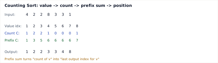
Worked example — Counting Sort on [4,2,2,8,3,3,1]
- Range: values 1..8, so k = 8. Count array C[1..8] initialized to 0.
- Tally: scan input → C = [1,2,2,1,0,0,0,1] (index i holds count of value i: 1→1, 2→2, 3→2, 4→1, 8→1).
- Prefix sum C in place → C = [1,3,5,6,6,6,6,7] (C[i] now = number of elements ≤ i, i.e. the last output index for value i, using 1-indexed positions).
- Scan input right to left (for stability) — original order is [4,2,2,8,3,3,1], so we visit 1, 3, 3, 8, 2, 2, 4: place 1 at index C[1]-1=0, decrement C[1]→0; place 3 at index C[3]-1=4, decrement C[3]→4; place 3 at index 3, decrement C[3]→3; place 8 at index C[8]-1=6, decrement C[8]→6; place 2 at index C[2]-1=2, decrement C[2]→2; place 2 at index 1, decrement C[2]→1; place 4 at index C[4]-1=5, decrement C[4]→5.
- Result: [1,2,2,3,3,4,8]. Check: every placement used the count value before decrementing as the 1-based rank, then decremented — the count array always holds "how many copies of this value remain to be placed," consistent with prefix sums meaning "last output index for this value."
Code — Counting Sort (Java)
static int[] countingSort(int[] arr, int maxVal) {
    int n = arr.length;
    int[] count = new int[maxVal + 1];
    for (int v : arr) count[v]++;
    for (int i = 1; i <= maxVal; i++) count[i] += count[i - 1]; // prefix sum
    int[] output = new int[n];
    for (int i = n - 1; i >= 0; i--) {           // right-to-left keeps it stable
        int v = arr[i];
        output[--count[v]] = v;
    }
    return output;
}
Pitfalls
- Ignoring the range k: Counting Sort on values up to 10⁹ with n = 100 allocates a 10⁹-entry array — blows memory and time despite being "O(n+k)".
- Negative numbers: naive count arrays assume value ≥ 0; must offset indices by min(arr) or the array indexes out of bounds.
- Left-to-right placement in Counting Sort: breaks stability — always place right-to-left when equal keys must preserve original order (needed for Radix Sort correctness, which relies on stability of each digit pass).
- Radix Sort digit direction: must process least-significant digit first; most-significant-first radix sort requires a different (recursive/bucketed) scheme entirely.
- Bucket Sort with skewed data: if the distribution is not roughly uniform, one bucket absorbs most elements and its internal sort dominates, degrading toward O(n log n) or worse.
When to use / when not
Use Counting/Radix Sort when keys are integers (or fixed-width encodable) and the range k or digit count d is small relative to n — e.g. sorting exam scores 0–100, sorting fixed-length employee IDs, or as the final radix pass in suffix-array construction. Use Bucket Sort when data is known to be uniformly distributed over a range (e.g. floats in [0,1)).
Avoid them when: keys are arbitrary objects with only a comparator (no extractable integer key), the range k is unbounded or huge relative to n, or memory is tightly constrained (O(k) or O(n) extra space is disqualifying).
Trade-off vs Quick Sort: Quick Sort is in-place (O(log n) space), works on any comparable type via a comparator, and has no dependency on key range — but averages O(n log n) and degrades to O(n²) worst case. Linear sorts trade that generality and worst-case comparison bound away for raw speed, at the cost of needing structural knowledge about the keys and extra memory.
Takeaways
- Linear sorts beat the Ω(n log n) comparison bound by using key values to compute positions directly, never comparing elements.
- Their true cost is O(n + k) or O(d·(n+b)) — the range/digit-count term is real and must be checked against n, not assumed small.
- Right-to-left placement in Counting Sort is what makes it stable, which is precisely what lets Radix Sort compose per-digit passes correctly.
- Choose linear sorts only when the key structure (bounded range, fixed width, uniform distribution) is confirmed — otherwise a comparison sort's generality wins.
Recall question
Why does sorting fixed-length 5-digit employee IDs with Radix Sort require each per-digit pass to be stable, and what breaks if one digit's pass is not stable?
Synthesized from CLRS (Counting Sort / Radix Sort chapter) and standard interview-prep treatments of linear-time sorting.
🤖 Don't fully get this? Learn it with Claude
Stuck on Introduction to Linear Sorting Algorithms? Open Claude, copy a block below, and it'll teach you this exact concept — visually and interactively.
Build the mental picture, not memorization.
I just read a lesson on **Introduction to Linear Sorting Algorithms** (DSA) and want to truly understand it. Explain Introduction to Linear Sorting Algorithms from first principles using ONE vivid real-world analogy and a visual mental model — draw it as ASCII art or a clear step-by-step diagram — with a concrete example using real numbers. Then ask me one question to check I got the mental picture, and wait for my reply. If you're unsure or a claim isn't standard, say so and reason from first principles instead of guessing.
Socratic — adapts to where you're stuck.
Teach me **Introduction to Linear Sorting Algorithms** interactively. Ask me ONE guiding question at a time, wait for my answer, and adapt to my confusion — build the idea with me step by step instead of explaining it all at once. If you're unsure or a claim isn't standard, say so and reason from first principles instead of guessing.
Active recall exposes what you missed.
Quiz me on **Introduction to Linear Sorting Algorithms** with 5 questions, easy to tricky, ONE at a time. Tell me if each answer is right; at the end, explain clearly what I got wrong and why. If you're unsure or a claim isn't standard, say so and reason from first principles instead of guessing.
Intuition + hook + flashcards for long-term memory.
Help me remember **Introduction to Linear Sorting Algorithms** for the long term: give the one-sentence intuition, a memorable hook/mnemonic, a tiny worked example, and 3 active-recall flashcards (Q -> A). If you're unsure or a claim isn't standard, say so and reason from first principles instead of guessing.