Counting Sort Algorithm
Counting Sort
Counting sort avoids comparisons altogether: it counts how many times each key value occurs, converts those counts into cumulative counts ("how many elements are ≤ this value"), and uses that cumulative count directly as the final index of each element — turning sorting into an array-indexing problem instead of an ordering problem.
Recognize the pattern
- Keys are integers (or cheaply mappable to integers) in a range
[0, k]that is not much larger thann. - You need a stable sort — equal keys must keep their relative input order (this matters when counting sort is used as a subroutine of radix sort).
- The problem hints at a bounded/known domain: "ages 0–120", "grades 0–100", "digits 0–9", "scores capped at k".
- You must beat O(n log n) and the data is discrete and bounded, not arbitrary comparable objects.
Brute force → optimal
Brute force: a comparison sort (merge sort, quicksort) treats elements as opaque and only asks "is a < b?". That costs O(n log n) comparisons and time, ignoring the fact that the values are small bounded integers.
Optimal (counting sort): tally frequencies in an array indexed by value, prefix-sum the tallies into placement offsets, then place each element once using those offsets. Cost drops to O(n + k) time at the price of O(k) extra space — it only applies to bounded integer keys, not general comparable objects.
Complexity, derived from first principles
Let n = number of elements. The Java implementation below assumes non-negative keys and sizes the count array as max + 1 with no min-offset, so for that code k = max + 1 — the value itself is the index. (The offset variant shown in Pitfalls instead uses k = max−min+1; the two are different implementations with different k, not the same code with two derivations.)
- Find max: one pass → O(n).
- Allocate and zero the count array: k writes, O(k).
- Tally frequencies: one pass over input, one increment per element → O(n).
- Prefix-sum the count array: one pass over k buckets, one addition each → O(k).
- Place elements (stable, traversed in reverse): one pass over input, one array write and one decrement per element → O(n).
- Copy output back: O(n).
Total time = O(n) + O(k) + O(n) + O(k) + O(n) + O(n) = O(n + k). This beats the O(n log n) comparison lower bound because counting sort never compares two elements — the lower bound only binds algorithms that make ordering decisions via comparisons.
Space: count array O(k), output array O(n) → O(n + k) auxiliary space (not in-place). When k ≫ n, the count array dominates and the algorithm becomes worse than O(n log n). This is why an input like [100000, 100001, 100002] is dangerous for the plain implementation below: it allocates new int[100003] and runs in O(n + max), not O(n + range) — the range is only 3, but nothing in that code exploits it. Only the offset variant in Pitfalls achieves O(n + (max−min+1)) on such input.
Traced example
Input: [4, 2, 2, 8, 3, 3, 1], n = 7, max = 8, so count array has size 9 (indices 0..8).
| Step | State |
|---|---|
| Tally | count = [0,1,2,2,1,0,0,0,1] (index i holds how many times value i appears: 1→1, 2→2, 3→2, 4→1, 8→1) |
| Prefix sum | count = [0,1,3,5,6,6,6,6,7] (count[v] = number of elements ≤ v = last output index for value v) |
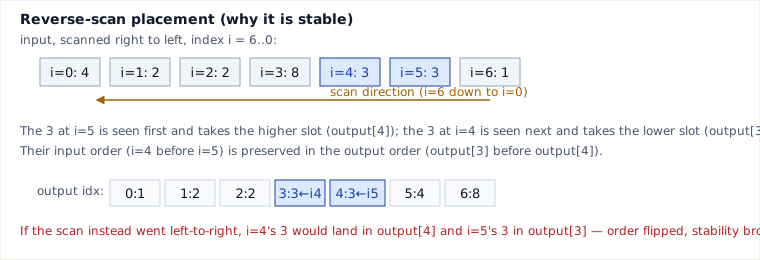
Placing elements by scanning the input right-to-left (this is what preserves stability):
| i | val | action | output after | count after |
|---|---|---|---|---|
| 6 | 1 | place at count[1]-1=0 | [1,_,_,_,_,_,_] | count[1]→0 |
| 5 | 3 | place at count[3]-1=4 | [1,_,_,_,3,_,_] | count[3]→4 |
| 4 | 3 | place at count[3]-1=3 | [1,_,_,3,3,_,_] | count[3]→3 |
| 3 | 8 | place at count[8]-1=6 | [1,_,_,3,3,_,8] | count[8]→6 |
| 2 | 2 | place at count[2]-1=2 | [1,_,2,3,3,_,8] | count[2]→2 |
| 1 | 2 | place at count[2]-1=1 | [1,2,2,3,3,_,8] | count[2]→1 |
| 0 | 4 | place at count[4]-1=5 | [1,2,2,3,3,4,8] | count[4]→5 |
Final sorted output: [1, 2, 2, 3, 3, 4, 8]. Note the two 2's (input indices 2,1) and two 3's (input indices 5,4) retained their original relative order — that is stability, produced by scanning the input right-to-left.
Java implementation
static int[] countingSort(int[] arr) {
    if (arr.length == 0) return arr;
    int max = arr[0];
    for (int v : arr) max = Math.max(max, v);
    int[] count = new int[max + 1];
    for (int v : arr) count[v]++;
    for (int i = 1; i <= max; i++) count[i] += count[i - 1]; // cumulative
    int[] output = new int[arr.length];
    for (int i = arr.length - 1; i >= 0; i--) {   // reverse scan => stable
        output[count[arr[i]] - 1] = arr[i];
        count[arr[i]]--;
    }
    return output;
}
This version only handles non-negative keys and its cost is O(n + max), because it never subtracts a min offset — see the offset variant below for the O(n + (max−min+1)) version.
Pitfalls
- Negative numbers / large min: the implementation above is indexed directly by value (size max+1), so it can't handle negative keys, and it wastes space when min is far from 0 (e.g.
[100000, 100001, 100002]allocates 100003 slots for 3 elements). Fix: offset every key by-minbefore indexing, and add min back when writing to output.
This is the version that actually achieves O(n + k) with k = max−min+1 for arbitrary integer ranges, including negatives and large offsets — onstatic int[] countingSortOffset(int[] arr) { if (arr.length == 0) return arr; int min = arr[0], max = arr[0]; for (int v : arr) { min = Math.min(min, v); max = Math.max(max, v); } int k = max - min + 1; int[] count = new int[k]; for (int v : arr) count[v - min]++; for (int i = 1; i < k; i++) count[i] += count[i - 1]; int[] output = new int[arr.length]; for (int i = arr.length - 1; i >= 0; i--) { output[count[arr[i] - min] - 1] = arr[i]; count[arr[i] - min]--; } return output; }[100000, 100001, 100002]it allocates only 3 slots, not 100003. - Unbounded / huge range: if k is much bigger than n (e.g. sorting 10 random 32-bit ints), the count array allocation alone destroys the linear-time benefit and can exhaust memory, even with the offset variant.
- Forgetting the reverse scan: placing elements left-to-right with a naively decremented count array still sorts correctly but reverses the relative order of equal keys — silently breaks stability, which breaks radix sort correctness.
- Off-by-one in cumulative counts: using
count[key]instead ofcount[key]-1as the index is the most common bug — write the position, then decrement. - Not applicable to floating-point or arbitrary objects without a quantization/mapping step.
When to use / when not — trade-offs vs Radix Sort
Use counting sort when keys are integers with a range k = O(n) (or smaller), you need stability, and you want guaranteed linear time regardless of input order (unlike quicksort's O(n²) worst case).
Avoid it when the key range is large relative to n, keys aren't integers/discretizable, or memory is tight (O(k) auxiliary space is non-negotiable).
vs. Radix Sort: radix sort decomposes a large-range integer (or string) key into fixed-width digits and runs counting sort once per digit, achieving O(d·(n+b)) for d digits of base b — this is the right choice when k is too large for one counting-sort pass but keys have bounded digit-length (e.g. 32-bit ints, fixed-length strings). Counting sort is radix sort's stable building block, not its competitor.
vs. comparison sorts (merge/quicksort): comparison sorts handle arbitrary orderable types and use O(n) extra space (merge sort) or O(log n) (quicksort), at O(n log n) time; counting sort trades that generality for O(n+k) time when its preconditions hold.
Takeaways
- Counting sort replaces comparisons with direct indexing: cumulative counts encode final positions.
- Its O(n+k) time and O(n+k) space are only good when k is not much larger than n — always check the range, and offset by min when keys aren't already near zero.
- Scanning the input in reverse while placing elements is what makes it stable, and that stability is exactly what radix sort depends on.
Recall question
Given the count array after the cumulative-sum step, why does traversing the input right-to-left (rather than left-to-right) preserve the relative order of equal keys in the output?
Synthesized and deepened from the original page source and standard CLRS-style counting sort treatment.
🤖 Don't fully get this? Learn it with Claude
Stuck on Counting Sort Algorithm? Open Claude, copy a block below, and it'll teach you this exact concept — visually and interactively.
Build the mental picture, not memorization.
I just read a lesson on **Counting Sort Algorithm** (DSA) and want to truly understand it. Explain Counting Sort Algorithm from first principles using ONE vivid real-world analogy and a visual mental model — draw it as ASCII art or a clear step-by-step diagram — with a concrete example using real numbers. Then ask me one question to check I got the mental picture, and wait for my reply. If you're unsure or a claim isn't standard, say so and reason from first principles instead of guessing.
Socratic — adapts to where you're stuck.
Teach me **Counting Sort Algorithm** interactively. Ask me ONE guiding question at a time, wait for my answer, and adapt to my confusion — build the idea with me step by step instead of explaining it all at once. If you're unsure or a claim isn't standard, say so and reason from first principles instead of guessing.
Active recall exposes what you missed.
Quiz me on **Counting Sort Algorithm** with 5 questions, easy to tricky, ONE at a time. Tell me if each answer is right; at the end, explain clearly what I got wrong and why. If you're unsure or a claim isn't standard, say so and reason from first principles instead of guessing.
Intuition + hook + flashcards for long-term memory.
Help me remember **Counting Sort Algorithm** for the long term: give the one-sentence intuition, a memorable hook/mnemonic, a tiny worked example, and 3 active-recall flashcards (Q -> A). If you're unsure or a claim isn't standard, say so and reason from first principles instead of guessing.