Bucket Sort Algorithm
Mechanism
Bucket sort speeds past the comparison-sort floor of O(n log n) by first using the values themselves as an approximate address: it scatters n elements into buckets keyed by value range, so that if the input is drawn from a roughly uniform distribution, each bucket ends up with only a small number of elements on average. Sorting many small sub-lists and concatenating them in bucket order is then cheaper than sorting the whole array as one comparison problem. How much cheaper depends directly on how many buckets you use — that choice is a real time/space knob, not a free lunch, as the derivation below makes explicit.
Recognize the pattern
- Input is numeric (or otherwise has a total order with a known/estimable min–max range) and is roughly uniformly distributed — not adversarial or heavily skewed.
- You know or can cheaply compute the range (min, max) up front, so you can map value → bucket index in O(1).
- The problem hints at 'floats in [0,1)', 'ages', 'scores', or explicitly says the data is uniform/random — that's the tell distinguishing it from counting sort (small integer range, no distribution assumption needed) or radix sort (fixed-width keys, digit-based).
Brute force → optimal
Brute force: any comparison sort (merge sort, quicksort, heapsort) treats every element as equally likely to be compared against every other — cost O(n log n) time, no assumption about the data needed, always correct.
Bucket sort exploits the distribution assumption, but how much it wins by depends on the number of buckets k, and that is a genuine space/time trade-off, not a fixed constant: pushing k up toward Θ(n) buys expected linear time at the cost of Θ(n) extra space for the bucket structures; pulling k down toward Θ(√n) — as the reference implementation below does — cuts that space to Θ(√n) but, as derived next, gives up the linear-time guarantee.
Complexity, derived (for the implementation actually shown below)
Setup: creating k empty buckets costs Θ(k).
Distribution: one pass over n elements, O(1) index computation each → Θ(n).
Per-bucket sort — matched to the code, which uses Collections.sort (TimSort, O(m log m) for a bucket of size m), not insertion sort: the reference implementation sets numBuckets = ⌊√n⌋, so k = √n and expected bucket size is n/k = √n (via the standard balls-into-bins argument: with n balls uniform over k bins, E[bin size] = n/k, and this holds whether k is n or √n — only the resulting bucket size changes). Summing the per-bucket TimSort cost across all k ≈ √n buckets, each expected to hold ≈ √n elements: total ≈ k · O((n/k) log(n/k)) = O(n · log(n/k)). With k = √n, log(n/k) = log(√n) = (log n)/2, so this is Θ(n log n).
Concatenation: Θ(n).
Total expected time for THIS code (k = Θ(√n), Collections.sort per bucket): Θ(n log n) — asymptotically no better than a plain comparison sort, though typically faster in practice by a constant factor since each Collections.sort call operates on a much smaller list. This is the direct consequence of the k choice: had the implementation instead used numBuckets = Θ(n) (so expected bucket size is O(1), and sorting O(1) elements is O(1) each), the same balls-into-bins math gives total expected time Θ(n) — but at the cost of Θ(n) extra space for bucket bookkeeping instead of Θ(√n). √n buckets is a deliberate space-for-time trade: less memory, but the expected-linear-time property is lost. (A from-scratch insertion sort per bucket, for comparison, costs O(k_i²) per bucket; summed via E[Σk_i²] = n + n(n-1)/k, that hits Θ(n) only when k = Θ(n) — again consistent with the space/time story, but that is not the sort used in the code below.)
Worst case: all n elements land in one bucket (e.g., all equal, or a skewed/adversarial distribution) → that bucket's Collections.sort costs O(n log n) — same order as the expected case here, so skew doesn't change the asymptotic class for this k, though it does erase any constant-factor win from smaller sub-lists.
Space: Θ(n + k) = Θ(n + √n) = Θ(n) for the buckets themselves (not in-place) — dominated by the n elements stored across buckets, with the √n bucket-list overhead being the part this k choice minimizes relative to a k = Θ(n) design.
Worked example
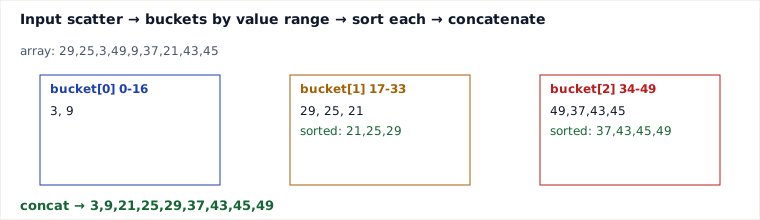
array = [29, 25, 3, 49, 9, 37, 21, 43, 45], n = 9, numBuckets = ⌊√9⌋ = 3, maxVal = 49. Index formula: bucketIndex = (num * numBuckets) / (maxVal + 1) = (num * 3) / 50 (integer division). With n this small the Θ(n log n) vs Θ(n) gap isn't visible numerically — the point of this example is to trace the mechanics (index computation, distribution, per-bucket TimSort, concatenation), not to demonstrate asymptotic behavior, which only shows up at scale.
| num | num*3 | /50 | bucket |
|---|---|---|---|
| 29 | 87 | 1 | 1 |
| 25 | 75 | 1 | 1 |
| 3 | 9 | 0 | 0 |
| 49 | 147 | 2 | 2 |
| 9 | 27 | 0 | 0 |
| 37 | 111 | 2 | 2 |
| 21 | 63 | 1 | 1 |
| 43 | 129 | 2 | 2 |
| 45 | 135 | 2 | 2 |
Buckets after distribution: [0]=[3,9], [1]=[29,25,21], [2]=[49,37,43,45]. After sorting each (Collections.sort): [0]=[3,9], [1]=[21,25,29], [2]=[37,43,45,49]. Concatenated result: [3, 9, 21, 25, 29, 37, 43, 45, 49].
Reference implementation (Java)
import java.util.*;

class BucketSort {
    static void sort(int[] arr) {
        int n = arr.length;
        if (n <= 1) return;
        int max = Arrays.stream(arr).max().getAsInt();
        int numBuckets = Math.max(1, (int) Math.sqrt(n)); // k = Θ(√n): trades expected-linear time for Θ(√n) space
        List> buckets = new ArrayList<>();
        for (int i = 0; i < numBuckets; i++) buckets.add(new ArrayList<>());

        for (int num : arr) {
            int idx = (int) ((long) num * numBuckets / (max + 1));
            buckets.get(idx).add(num);
        }
        int pos = 0;
        for (List bucket : buckets) {
            Collections.sort(bucket); // TimSort, O(m log m) per bucket of size m
            for (int v : bucket) arr[pos++] = v;
        }
    }
}
With this k and this per-bucket sort, expected total time is Θ(n log n) (derived above) — not Θ(n). To recover expected-linear time, set numBuckets to Θ(n) (e.g. = n) instead of √n; that raises bucket-structure space from Θ(√n) to Θ(n).
Pitfalls
- Assuming 'bucket sort' always means Θ(n): the Θ(n) expected bound requires k = Θ(n) buckets AND near-O(1) work per bucket. Fewer buckets (e.g. √n, as above) or a comparison-based per-bucket sort each independently erode that bound — combined, as in the code here, the honest bound is Θ(n log n), not Θ(n).
- Skewed input collapses buckets: if data clusters (e.g. many duplicates or an exponential distribution), one bucket absorbs most elements and per-bucket sort dominates — O(n log n) here (TimSort on ~n elements), or O(n²) if the per-bucket sort were insertion sort instead.
- Off-by-one index overflow: using max value alone (without +1) can push the maximum element into an out-of-range bucket index; also watch integer overflow when num*numBuckets is computed for large ints (use long as shown above).
- Wasted buckets on small/negative-range data: negative numbers need an offset (shift by -min) before indexing, and a tiny value range vs many buckets wastes memory with mostly-empty buckets.
- Assuming stability: bucket sort is stable only if both the distribution and the per-bucket sort are stable —
Collections.sortis stable, but swapping in a non-stable per-bucket sort (e.g. quicksort) breaks that guarantee silently.
When to use / when not
Use when data is numeric, roughly uniformly distributed over a known range, and you deliberately size k: pick k = Θ(n) if you need expected-linear time and can afford Θ(n) bucket-structure space; pick k = Θ(√n) (as in the reference code) if you want to trade that time bound down to Θ(n log n) expected in exchange for Θ(√n) space instead.
Avoid when the distribution is unknown or adversarial, or data isn't easily bucketable by value.
| Approach | Time | Space | Assumption |
|---|---|---|---|
| Bucket sort, k=Θ(n) | Θ(n) expected, O(n²) worst (insertion sort per bucket) | Θ(n) | uniform distribution, known range |
| Bucket sort, k=Θ(√n) (this page's code) | Θ(n log n) expected and worst (TimSort per bucket) | Θ(n) total, Θ(√n) bucket overhead | uniform distribution, known range |
| Merge/Heap sort | Θ(n log n) always | O(n) / O(1) | none (comparison-based) |
| Counting sort | Θ(n + range) | O(range) | small integer range |
| Radix sort | Θ(d·(n+b)) | O(n+b) | fixed-width keys, digit base b |
Takeaways
- Bucket sort's headline Θ(n) claim is conditional on TWO choices, not one: k = Θ(n) buckets AND O(1)-ish work per bucket. Change either — as the reference code does by using k = Θ(√n) with a comparison-based Collections.sort — and the honest bound becomes Θ(n log n), not Θ(n).
- The number of buckets is a real space/time dial: more buckets (up to Θ(n)) buys expected-linear time at Θ(n) space; fewer buckets (down to Θ(√n)) shrinks bucket-structure space to Θ(√n) but gives that time bound back up.
- It is not a comparison sort at the top level — comparisons only happen inside buckets — but if those buckets are large enough for their internal comparison sort to dominate (as with k=√n), the overall guarantee collapses back to the n log n class, just with better constants.
Recall: If the reference implementation above is run on 1000 elements that are all identical, what is the resulting time complexity, and why does it match the derived worst case rather than degrade further?
Synthesized from the source extract's step-by-step walkthrough and complexity notes, cross-checked against standard bucket-sort analysis (balls-into-bins expectation) and CLRS-style treatment of distribution sorts; the complexity derivation was re-worked here to match the reference implementation's actual bucket count (Θ(√n)) and per-bucket sort (TimSort via Collections.sort) rather than the idealized k=Θ(n)/insertion-sort textbook case.
🤖 Don't fully get this? Learn it with Claude
Stuck on Bucket Sort Algorithm? Open Claude, copy a block below, and it'll teach you this exact concept — visually and interactively.
Build the mental picture, not memorization.
I just read a lesson on **Bucket Sort Algorithm** (DSA) and want to truly understand it. Explain Bucket Sort Algorithm from first principles using ONE vivid real-world analogy and a visual mental model — draw it as ASCII art or a clear step-by-step diagram — with a concrete example using real numbers. Then ask me one question to check I got the mental picture, and wait for my reply. If you're unsure or a claim isn't standard, say so and reason from first principles instead of guessing.
Socratic — adapts to where you're stuck.
Teach me **Bucket Sort Algorithm** interactively. Ask me ONE guiding question at a time, wait for my answer, and adapt to my confusion — build the idea with me step by step instead of explaining it all at once. If you're unsure or a claim isn't standard, say so and reason from first principles instead of guessing.
Active recall exposes what you missed.
Quiz me on **Bucket Sort Algorithm** with 5 questions, easy to tricky, ONE at a time. Tell me if each answer is right; at the end, explain clearly what I got wrong and why. If you're unsure or a claim isn't standard, say so and reason from first principles instead of guessing.
Intuition + hook + flashcards for long-term memory.
Help me remember **Bucket Sort Algorithm** for the long term: give the one-sentence intuition, a memorable hook/mnemonic, a tiny worked example, and 3 active-recall flashcards (Q -> A). If you're unsure or a claim isn't standard, say so and reason from first principles instead of guessing.