Latency vs Throughput
Latency is the time one request spends in the system; throughput is how many requests complete per second — and they are not two independent knobs. Little's Law (L = λW) and queueing theory bolt them together: a system holds L requests in flight, admits λ per second, and each spends W inside. Fix any two and the third is forced. That coupling is why "just push more load" eventually wrecks response time, and why batching for throughput always taxes latency.
The definitions are the easy part: latency is measured in time (ms), throughput in work per time (req/s, rows/s, MB/s). The engineering is understanding the relationship — how one moves when you chase the other.
Little's Law: the leash between them
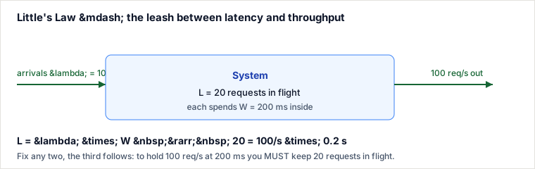
For any stable system (nothing piling up forever), the average number of requests in flight equals the arrival rate times the time each spends inside:
L = λ × W (concurrency = throughput × latency)
This holds regardless of internal structure — no assumption about the arrival pattern or service distribution. It is the reason latency and throughput cannot both be chosen freely under a fixed concurrency budget.
Worked example. One request takes W = 200 ms. On a single thread only one request is in flight (L = 1), so throughput is capped at λ = L / W = 1 / 0.2 s = 5 req/s — no matter how fast the network is. To reach 100 req/s at that same 200 ms latency you must keep L = λW = 100 × 0.2 = 20 requests in flight (20 threads, or 20 async connections). Conversely, if you only have 20 slots and want 100 req/s, you must drive latency down to 200 ms or lower. Throughput, latency, concurrency — pick two, the third is decided.
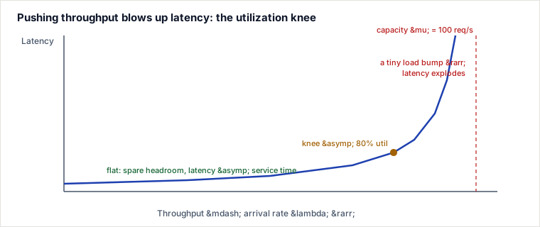
The utilization knee: why chasing throughput explodes latency
Little's Law says the numbers must balance; queueing theory says how latency reacts as you approach capacity. Model a single server that can complete μ requests/s (service time 1/μ) receiving λ requests/s. Utilization is ρ = λ / μ. For a simple M/M/1 queue, mean response time is:
W = (1/μ) / (1 − ρ)
The 1 − ρ in the denominator is the whole story: as offered load approaches capacity, response time doesn't rise linearly — it goes vertical. With a 10 ms service time (μ = 100 req/s):
| Load λ (req/s) | Utilization ρ | Mean latency W |
|---|---|---|
| 50 | 0.50 | 20 ms |
| 80 | 0.80 | 50 ms |
| 90 | 0.90 | 100 ms |
| 95 | 0.95 | 200 ms |
| 99 | 0.99 | 1000 ms |
Going from 50 to 99 req/s — a 2× throughput gain — costs a 50× latency increase. Past roughly 70–80% utilization you are on the steep wall: a tiny burst that nudges λ from 95 to 99 doubles latency again. This is why capacity planning targets utilization headroom (often ~50–70% for latency-sensitive tiers), not raw "can it handle it."
Batching: the classic trade, shown with numbers
The old note asserted "larger batches improve throughput but increase latency." Here is why, quantified. Suppose each database write batch has a fixed cost of 5 ms (network round trip + one fsync) plus 0.5 ms per row. Batching amortizes that fixed 5 ms across more rows, so throughput climbs — but every row now waits for the whole batch to be assembled and processed, so latency climbs too.
| Batch size b | Batch service = 5 + 0.5b | Throughput = b / service | Latency (one batch) |
|---|---|---|---|
| 1 | 5.5 ms | 182 rows/s | 5.5 ms |
| 10 | 10 ms | 1000 rows/s | 10 ms |
| 50 | 30 ms | 1667 rows/s | 30 ms |
| 100 | 55 ms | 1818 rows/s | 55 ms |
Throughput rose 10× (182 → 1818 rows/s) while per-request latency rose 10× (5.5 → 55 ms). Note the diminishing returns: from b=50 to b=100 you nearly double latency (30 → 55 ms) for a measly 9% more throughput, because the fixed 5 ms is already amortized away — throughput asymptotes at 1/0.5ms = 2000 rows/s no matter how big the batch. The same amortization mechanism drives Nagle's algorithm (TCP), Kafka's linger.ms, group commit in databases, and GPU inference batching. The knob is always "how much latency will I trade for the next slice of throughput?"
Pitfalls
- Running hot to "save money." Provisioning for 90–95% utilization looks efficient on a dashboard, but it parks you on the steep wall of the knee curve. A routine traffic bump or one slow dependency pushes ρ past 1, the queue grows unbounded, and latency goes to seconds. Latency-sensitive tiers need idle headroom by design.
- Optimizing the mean, shipping a terrible tail. Batching and high utilization inflate p99/p999 far more than the average. In a service that fans out to 100 backends, a request is as slow as its slowest call, so even a 1-in-100 tail event touches 1 − 0.99100 ≈ 63% of user-facing requests — the p99 of a component becomes roughly the median of the composed request. Measure p99, not just mean.
- Reporting throughput without concurrency. A load test with one client thread reporting "5 req/s" is measuring 1/W, not capacity. You cannot discover capacity without enough in-flight load (Little's Law again). Your load generator, not the system, may be the bottleneck.
- Coordinated omission. Closed-loop load tools that wait for a response before sending the next request stop sending during a stall — so the stall never appears in the latency histogram. Reported p99 looks great while real users are timing out. (See Gil Tene.)
- Adding threads to a saturated bottleneck. Past the Little's-Law point, more threads don't raise throughput on a contended shared resource — they just lengthen the queue, so W rises to keep L = λW balanced, and contention/context-switching can make throughput drop (the Universal Scalability Law's retrograde region).
When to optimize for latency vs throughput
These pull in opposite directions, so pick per workload rather than globally.
Optimize for latency when a human or a tight SLA is waiting on each response: request/response web paths, checkout, search-as-you-type, gaming, ad bidding, high-frequency trading. Signals: p99 is in the SLO, requests are independent and user-blocking, revenue tracks responsiveness. Tactics: keep utilization at ~50–70%, minimize hops/serialization, avoid batching on the hot path, replicate for read-locality, keep headroom for bursts.
Optimize for throughput when the work is deferred or bulk and total time/$ per unit dominates: ETL, analytics, log/metric ingestion, backups, video transcoding, ML training, nightly reports. Signals: no user blocked on an individual item, cost-per-item matters, you can absorb queueing. Tactics: batch aggressively, run at 85–95% utilization, prefer sequential/vectorized processing, scale horizontally.
The named alternatives, and what each costs: A latency-optimized design buys predictable, low tail latency but costs money and utilization — you pay for idle headroom and give up amortization gains. A throughput-optimized design buys maximum work-per-dollar but costs responsiveness and tail predictability — queueing and batching push p99 up, and it sits closer to the cliff. Real systems split the difference: latency-critical traffic on a well-provisioned interactive tier, and a separate throughput-tier (queue + batch workers) for everything that can wait. Choose latency-first when a person is blocked on the answer; choose throughput-first when a machine will consume the result later.
Takeaways
- They're coupled, not independent: L = λW means concurrency, throughput, and latency form a triangle — you can only choose two.
- Latency is roughly flat until the knee, then vertical: W = (1/μ)/(1−ρ). Protect latency-sensitive tiers by leaving utilization headroom (~50–70%).
- Every throughput trick taxes latency: batching, high utilization, and deep queues raise work-per-second and per-request delay together, with diminishing throughput returns.
- Design per workload: latency-first when a person waits on each answer; throughput-first when a machine consumes the result later — and measure the tail (p99), not the mean.
Re-authored/Deepened for this guide. Sources: J. D. C. Little, "A Proof for the Queuing Formula: L = λW" (Operations Research, 1961); L. Kleinrock, Queueing Systems (M/M/1 response-time analysis); Neil Gunther, Guerrilla Capacity Planning (Universal Scalability Law); Gil Tene, "How NOT to Measure Latency" (coordinated omission, tail latency); Brendan Gregg, Systems Performance (utilization and the USE method); Martin Kleppmann, Designing Data-Intensive Applications, ch. 1 (percentiles and tail latency amplification).
🤖 Don't fully get this? Learn it with Claude
Stuck on Latency vs Throughput? Open Claude, copy a block below, and it'll teach you this exact concept — visually and interactively.
Build the mental picture, not memorization.
I just read a lesson on **Latency vs Throughput** (System Design) and want to truly understand it. Explain Latency vs Throughput from first principles using ONE vivid real-world analogy and a visual mental model — draw it as ASCII art or a clear step-by-step diagram — with a concrete example using real numbers. Then ask me one question to check I got the mental picture, and wait for my reply. If you're unsure or a claim isn't standard, say so and reason from first principles instead of guessing.
Socratic — adapts to where you're stuck.
Teach me **Latency vs Throughput** interactively. Ask me ONE guiding question at a time, wait for my answer, and adapt to my confusion — build the idea with me step by step instead of explaining it all at once. If you're unsure or a claim isn't standard, say so and reason from first principles instead of guessing.
Active recall exposes what you missed.
Quiz me on **Latency vs Throughput** with 5 questions, easy to tricky, ONE at a time. Tell me if each answer is right; at the end, explain clearly what I got wrong and why. If you're unsure or a claim isn't standard, say so and reason from first principles instead of guessing.
Intuition + hook + flashcards for long-term memory.
Help me remember **Latency vs Throughput** for the long term: give the one-sentence intuition, a memorable hook/mnemonic, a tiny worked example, and 3 active-recall flashcards (Q -> A). If you're unsure or a claim isn't standard, say so and reason from first principles instead of guessing.