NoSQL Databases

NoSQL ("Not Only SQL") is an umbrella term for databases that deliberately step away from the strict relational model you met in Introduction to Databases (001). Where a relational engine forces every row into a fixed table schema and reaches consistency through ACID transactions, NoSQL systems trade some of those guarantees for three things applications at scale often need more: a flexible or absent schema, horizontal scalability across commodity machines, and shape-specific performance for one dominant access pattern.

The important mental shift: NoSQL is not one technology. It is a family of five or six distinct data models, each optimized for a different question. Choosing "a NoSQL database" is meaningless until you say which model, because a graph database and a wide-column database are as different from each other as either is from PostgreSQL.

The six data models

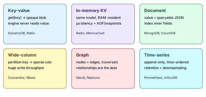
NoSQL stores are conventionally grouped into six families. The first two are closely related (in-memory key-value is a specialization of key-value), which is why some texts collapse the list to five — but the access patterns are distinct enough to treat separately.

1. Key-value — an opaque value addressed by a unique key. Fastest possible point lookups; the database never looks inside the value. Examples: Amazon DynamoDB, Azure Cosmos DB, Redis.
2. In-memory key-value — the same model with the working set held in RAM for microsecond latency, optionally persisted via an append-only log or periodic snapshots. Examples: Redis, Memcached, Amazon ElastiCache.
3. Document — key-value where the value is a structured document (JSON/BSON/XML) the engine can query and index by its inner fields. Examples: MongoDB, Amazon DocumentDB, CouchDB.
4. Wide-column — rows keyed by a partition key, with a flexible, sparse set of columns per row; tuned for enormous write throughput and predictable partition-scoped reads. Examples: Apache Cassandra, HBase, Azure Table Storage.
5. Graph — nodes and edges as first-class citizens, optimized for traversing relationships. Examples: Neo4j, Amazon Neptune, Cosmos DB (Gremlin API).
6. Time-series — append-heavy streams ordered by timestamp, with built-in retention, downsampling, and time-window aggregation. Examples: Prometheus, InfluxDB, Amazon Timestream, Graphite.

A note on graph traversal cost

Graph databases are worth a closer look because their headline performance claim is model-specific. Neo4j uses index-free adjacency: each node stores direct physical pointers to its incident relationships, so hopping from a node to its neighbors is a pointer chase rather than an index lookup. A k-hop traversal therefore costs roughly O(hops × average degree) and is independent of the total graph size — the property that makes deep traversals ("friends of friends of friends") fast.

This is a property of Neo4j specifically, not of the graph model in general. Amazon Neptune, despite being a graph database, is an indexed engine — it resolves adjacency through indexed lookups rather than index-free adjacency, so its traversal-cost characteristics differ. Treat "index-free adjacency" as a Neo4j feature you can lean on, and verify the engine before assuming any specific graph store has it.

Worked example: a chat app on Cassandra

Abstract taxonomies don't build intuition — modeling one real table does. We'll store chat messages in Apache Cassandra (wide-column) and watch how its query-first design shapes every decision. In Cassandra you design the table around the query you must serve, not around normalized entities.

Our dominant query is "show the recent messages in a room, newest first." That single sentence dictates the schema:

CREATE TABLE messages (
  room_id   int,
  sent_at   timestamp,
  author    text,
  body      text,
  PRIMARY KEY (room_id, sent_at)
) WITH CLUSTERING ORDER BY (sent_at DESC);

The primary key has two parts. room_id is the partition key — it decides which node owns the data. sent_at is the clustering column — it decides the on-disk sort order within a partition. CLUSTERING ORDER BY (sent_at DESC) physically stores each room's messages newest-first, so our dominant query reads sequentially with no sort step.

The write path

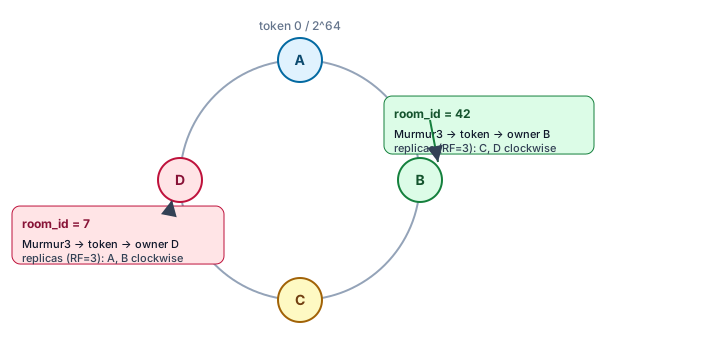
When we insert a row, Cassandra hashes the partition key with Murmur3 to produce a 64-bit token, then walks the ring clockwise to the node that owns that token range (and, for replication factor 3, the next two nodes clockwise). All messages for room_id = 42 land on the same partition on the same owner node, which is exactly why reading one room is a single-node, single-partition operation.

Note the CQL below: unlike SQL, CQL has no columnless INSERT form — the column list is mandatory. Cassandra timestamps also require a full date-and-time literal (ISO-8601 or epoch millis); a bare '09:01' will not parse.

INSERT INTO messages (room_id, sent_at, author, body)
  VALUES (42, '2024-01-01 09:01:00', 'alice', 'standup?');
INSERT INTO messages (room_id, sent_at, author, body)
  VALUES (42, '2024-01-01 09:02:00', 'bob',   'omw');
INSERT INTO messages (room_id, sent_at, author, body)
  VALUES (42, '2024-01-01 09:03:00', 'alice', 'joining now');
INSERT INTO messages (room_id, sent_at, author, body)
  VALUES (7,  '2024-01-01 09:01:30', 'carol', 'hi room 7');

Why wide-column is write-fast: the LSM tree

The "enormous write throughput" claim is not marketing — it falls directly out of the storage engine. Cassandra (like HBase, RocksDB, and LevelDB) is built on a log-structured merge-tree (LSM tree), and the defining property is that it never updates data in place. A write takes exactly two cheap steps:

1. Append to the commit log — a sequential write to an on-disk append-only log, purely for durability (crash recovery).
2. Insert into the memtable — an in-memory sorted structure (e.g. a balanced tree / skiplist) holding recent writes for this table.

That is the entire write path. When a memtable fills, it is flushed as-is to disk as an immutable, sorted file called an SSTable (sorted string table) and a fresh memtable takes over. Crucially there is no read-before-write: the engine never has to locate and rewrite an existing row the way a B-tree does. Every write is a sequential append plus an in-memory insert, so write cost is roughly O(1) and disk I/O is sequential (fast) rather than random (slow) — which is exactly why the model sustains huge write rates.

The bill arrives on reads. A single key can live in the memtable or in any of several SSTables written at different times (plus tombstones for deletes), so a read may have to consult multiple files and merge the results by timestamp — this is read amplification. Two mechanisms keep it bounded: a per-SSTable bloom filter lets a read skip files that certainly do not contain the key (pruning most, though not all, of the fan-out), and background compaction continuously merges SSTables together, discarding superseded values and tombstones so the number of files a read must touch stays small. Compaction is real, ongoing write and I/O work — the deferred cost of never paying for in-place updates up front.

This is the LSM trade in one line, and it is the mirror image of a classic relational store: Postgres/MySQL use B-trees and update in place — reads touch one location (read-optimized) but writes must find and rewrite a page, sometimes triggering random I/O (write-costlier). Cassandra's LSM inverts that: cheap sequential writes, at the cost of read amplification and continuous compaction. Choose wide-column when the workload is write-dominant and the read patterns are known; choose a B-tree store when reads are the hot path and you need in-place update economics.

Trace one row through it: INSERT ... room_id=42 → appended to the commit log → inserted into the memtable. Minutes later the memtable flushes to SSTable-3. Now a SELECT ... WHERE room_id=42 checks the current memtable, then — guided by bloom filters — SSTable-3, SSTable-2, SSTable-1, merging matching rows newest-wins; compaction will later fold those SSTables into one so the same read touches fewer files.

The read path — and where it bites

Because room_id is the partition key, the query the schema was built for is trivial and fast — Cassandra hashes 42, goes straight to the owning node, and streams the partition in stored order:

SELECT * FROM messages WHERE room_id = 42;
-- room 42, newest first: 'joining now', 'omw', 'standup?'

You can also slice within the partition using the clustering column, still touching only one partition:

SELECT * FROM messages
  WHERE room_id = 42 AND sent_at > '2024-01-01 09:01:30';

Now the trap. Suppose product asks for "every message alice ever sent." author is not part of the primary key, so Cassandra has no way to locate the relevant partitions — the data for alice is scattered across every room, on every node. This query is rejected:

SELECT * FROM messages WHERE author = 'alice';
-- InvalidRequest: Cannot execute this query as it might involve
-- data filtering ... use ALLOW FILTERING

Appending ALLOW FILTERING makes it run — by scanning every partition on every node and discarding non-matches. That is O(all rows), degrades as the table grows, and is a well-known production anti-pattern. The correct fix is to model the second query as its own table (e.g. messages_by_author with author as the partition key) and write to both — trading storage and write amplification for fast reads. In Cassandra you duplicate data to serve queries; you do not filter your way to them.

Pitfalls that catch newcomers

• Modeling entities instead of queries. Relational habits say "one table per entity, join later." Wide-column and document stores punish this — design one table/collection per access pattern, even if it duplicates data.
• Unbounded partitions. A single room that accumulates millions of messages becomes one giant partition on one node — a hotspot. The standard remedy is bucketing: make the partition key (room_id, day) so each partition stays bounded.
• Trusting eventual consistency blindly. With replication and quorum tuning, a read right after a write may miss it. If you need read-your-writes, raise the consistency level (e.g. QUORUM reads + writes) and accept the latency cost.
• Reaching for secondary indexes and ALLOW FILTERING. Both exist, both look convenient, and both scale poorly for high-cardinality or cross-partition queries. Prefer a purpose-built query table.
• Expecting joins and multi-object transactions. Most NoSQL stores offer neither (or only limited, single-partition versions). Denormalization and application-level coordination replace them.

Choosing a model: selection and trade-offs

The judgment layer matters more than the taxonomy. For each model, the useful question is not "what is it" but "when does it beat the named alternative."

• Key-value (Redis, DynamoDB) vs. document (MongoDB). Choose key-value when every access is by primary key and the value is opaque to the database — sessions, feature flags, caches. Switch to a document store the moment you need to query inside the value ("find all orders over $100"); a key-value store cannot do that without scanning.
• Document (MongoDB) vs. relational (PostgreSQL). Choose document when your aggregate is self-contained and read/written as a unit (a user profile, a product page). Avoid it when the workload is heavy cross-entity JOINs and ad-hoc analytics — Postgres's optimizer and JSONB give you flexibility without giving up joins and constraints.
• Wide-column (Cassandra) vs. document (MongoDB). Choose Cassandra for extreme, always-on write throughput, multi-datacenter replication, and a small set of known query patterns. Avoid it when queries are exploratory or you need secondary access paths you can't predict — MongoDB's richer indexing is friendlier there.
• Graph (Neo4j) vs. recursive SQL joins. Choose a graph store when the core problem is deep, variable-length traversal (fraud rings, social distance, dependency chains); Neo4j's index-free adjacency keeps a k-hop traversal near O(hops × degree) regardless of total graph size. In a relational DB the same traversal degrades with each self-join. (If you're on Amazon Neptune instead, note it is index-backed rather than index-free, so validate traversal cost for your depth.)
• Time-series (Prometheus, InfluxDB, Timestream) vs. bolting timestamps onto a generic store. Choose a dedicated time-series engine when you ingest high-rate, append-only measurements and mostly ask time-window questions. You get retention policies, automatic downsampling, and time-bucketed aggregation for free — exactly the machinery you'd otherwise hand-build and get wrong on top of a generic store.

When to stay on SQL

NoSQL earns its complexity only when it solves a problem relational databases cannot. Prefer (or keep) SQL when: you need multi-object ACID transactions (banking, inventory, anything where partial commits corrupt state); your data is highly relational with frequent joins and aggregations; you're at modest scale where one well-tuned Postgres/MySQL node is plenty ("you are not Google"); you rely on ad-hoc analytics and BI; or you want the database itself to enforce schema and constraints rather than trusting application code.

The mature answer is often polyglot persistence: PostgreSQL for transactional core data, Redis for the cache, Cassandra or a time-series engine for high-volume telemetry, Neo4j for the recommendation graph — each technology doing only what it is best at. Start relational, and adopt a NoSQL model when you can name the concrete requirement it satisfies.

Sources & further reading

• Karan Pratap Singh, System Design — NoSQL Databases (github.com/karanpratapsingh/system-design), the base article this lesson expands.
• Apache Cassandra / DataStax CQL reference — mandatory column lists in INSERT, timestamp literal formats, and the semantics of ALLOW FILTERING (docs.datastax.com, cassandra.apache.org).
• Neo4j documentation — index-free adjacency and traversal cost (neo4j.com/docs); Amazon Neptune documentation for its indexed engine model (docs.aws.amazon.com/neptune).
• Martin Kleppmann, Designing Data-Intensive Applications (O'Reilly) — data models, partitioning, and consistency trade-offs underpinning the selection guidance above.

Interview drill ladder