Types of Indexes
An index works by keeping a copy of the indexed column(s) in a separate structure that is kept pre-sorted (a B-tree) or pre-hashed (a hash table), with the leaves pointing back at the table rows — so the engine can binary-search or hash straight to the matches instead of reading every page.
The "seven types" you will be asked about are not seven different data structures. Under the hood there are only three: the B-tree (ordered), the hash table (unordered, equality-only), and the inverted index (term → rows, for text). The other names describe two orthogonal properties layered on a B-tree — what role it plays (primary / unique = a B-tree plus a constraint) and whether it dictates the table's physical order (clustered vs non-clustered). "Composite" just means the B-tree key has more than one column. Hold that map and the catalog below stops being a list to memorise. How the B-tree and hash structures are actually built and traversed on disk is the subject of the next lesson, Storage Engines — How B-tree & LSM-tree Work; here we care about which kind of index to reach for and why.
The seven types at a glance
| Type | Underlying structure | Ordered? | Per table | Best for |
|---|---|---|---|---|
| Primary | B-tree + PK constraint | Yes | One | Exact lookup by identity; integrity |
| Unique | B-tree + uniqueness constraint | Yes | Many | Enforcing distinct values (email, SKU) |
| Clustered | B-tree that is the table | Yes | One | Range scans & sorting on the key |
| Non-clustered (secondary) | B-tree pointing at rows | Yes | Many | Selective filters & joins |
| Composite | B-tree with a multi-column key | Yes (by prefix) | Many | Multi-column filters / sorts |
| Full-text | Inverted index (term → rows) | By term | Many | Keyword / phrase search in text |
| Hash | Hash table | No | Engine-dependent | Equality-only lookups |
Notice that rows 1, 2, 4 and 5 all sit on the same B-tree machinery — only their role and key shape differ. Rows 3, 6 and 7 are where the physical structure actually changes.
Trace: one lookup through a secondary index
The single most important behaviour to internalise is what happens when you filter on a non-clustered index of a clustered table. Take a concrete InnoDB (MySQL) setup and follow one query byte for byte.
- Table
Customers: 2,000,000 rows, ~200 bytes each, on 16 KB pages ⇒ ~80 rows/page ⇒ ~25,000 leaf pages. - The table is clustered on its
PRIMARY KEYCustomerID— the row data lives in the leaves of the PK B-tree. - There is a secondary index
idx_emailonEmail. Both B-trees are 3 levels deep (root → internal → leaf).
Now run SELECT * FROM Customers WHERE Email = 'alice@example.com';
- Read 1 — secondary root. Compare
'alice@example.com'against the separator keys, pick a child. - Read 2 — secondary internal. Narrow again, descend to the right leaf.
- Read 3 — secondary leaf. Find the entry
('alice@example.com' → CustomerID = 8842). Crucial detail: in InnoDB a secondary-index leaf stores the primary key value, not a physical row pointer. We now know the row's identity but still have none of its columns. - Reads 4–6 — clustered index. Traverse the PK B-tree for
CustomerID = 8842: root → internal → leaf. The clustered leaf holds the full row, so we finally readNameandAddress.
That is 6 logical page reads to return one row — the classic "double lookup" (also called a bookmark lookup). Compare it to the alternative: a full table scan touches all ~25,000 leaf pages. Six versus twenty-five thousand is the entire reason indexes exist.
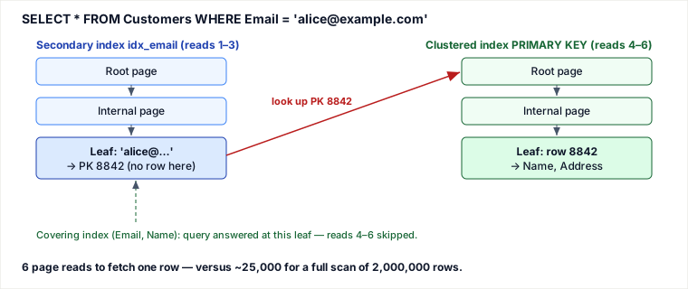
The second half of that trace (reads 4–6) is pure overhead you can sometimes delete. If the index already contains every column the query needs, the engine returns straight from the secondary leaf and never touches the clustered index — a covering index. Add Name to the key:
CREATE INDEX idx_email_name ON Customers (Email, Name);Now SELECT Name FROM Customers WHERE Email = 'alice@example.com' costs 3 reads, not 6. In MySQL's EXPLAIN you will see Using index; in Postgres, an Index Only Scan. The catch: a covering index is wider, so it costs more disk and more work on every write — you are trading write cost for read cost on one hot query.
One more thing the trace exposes: the engine can only seek when the predicate is sargable — the indexed column appears bare on one side of the comparison. WHERE YEAR(created_at) = 2024 or WHERE email = 12345 (type mismatch) wrap or coerce the column and force a scan; rewrite as WHERE created_at >= '2024-01-01' AND created_at < '2025-01-01'.
Primary and Unique — B-trees with a constraint
A primary index is the B-tree the database builds automatically for the PRIMARY KEY. It is unique, not-null, and — in InnoDB and SQL Server by default — it is also the clustered index, so it defines physical row order. One per table, because a table has one primary key.
A unique index is the same B-tree with a distinctness rule but no not-null/clustering implications; you can have many. Beyond speeding reads, it enforces integrity: every insert or key-update checks the tree for a duplicate before committing — a small, worth-it write cost.
CREATE TABLE Customers (
  CustomerID INT PRIMARY KEY,        -- primary (usually clustered) index
  Email      VARCHAR(255) NOT NULL,
  Name       VARCHAR(100)
);

CREATE UNIQUE INDEX idx_customers_email ON Customers (Email);
After this, a duplicate email is rejected and WHERE Email = ? resolves through the trace above.
Clustered vs Non-clustered — who owns the row
The distinction the trace hinges on. A clustered index stores the rows themselves in its leaves, sorted by the key — the index is the table. Only one per table (data can be physically sorted one way), and it makes range scans and ORDER BY on the key nearly free, because matching rows sit contiguously on disk.
A non-clustered (secondary) index is a lighter B-tree whose leaves hold the key plus a reference back to the row (the PK value in InnoDB, a physical row-id in a heap table like SQL Server without a clustered index or in Oracle). Many per table. Great for selective filters; poor when the predicate matches a large fraction of rows, where the optimizer will (correctly) prefer a full scan over thousands of random row fetches.
-- SQL Server: physically order the table by (LastName, FirstName)
CREATE CLUSTERED INDEX idx_cust_name ON Customers (LastName, FirstName);

-- A secondary index to accelerate a different access path
CREATE INDEX idx_orders_customer ON Orders (CustomerID);
Composite — the leftmost-prefix rule
A composite index keys on several columns treated as one concatenated sort key. The order of the columns is load-bearing: the engine can seek using a leading prefix only.
CREATE INDEX idx_orders_cust_date ON Orders (CustomerID, OrderDate);Against (CustomerID, OrderDate):
WHERE CustomerID = 42 AND OrderDate >= '2024-01-01' AND OrderDate < '2024-02-01'— full seek, both columns used.WHERE CustomerID = 42— seeks on the leading prefix. Fine.WHERE OrderDate >= '2024-01-01'alone — cannot seek;OrderDateis not the leading column. (Some engines mitigate with an index skip-scan, but treat that as a bonus, not a design assumption.)
So order the columns to match how you actually filter: equality columns first, then the range column. A common mistake is then adding a redundant single-column index on CustomerID — the composite already covers it.
Full-text — an inverted index for words
A B-tree keys on the whole column value, so LIKE '%database%' (a leading wildcard) cannot use it and falls back to a scan. A full-text index instead tokenises the text into words and builds an inverted index — each term maps to the rows containing it — enabling multi-word, phrase, and relevance-ranked search. Building and updating it is heavier (parsing, stop-word removal, stemming), often applied asynchronously, and it uses extra storage; queries need dedicated syntax.
-- MySQL / InnoDB
CREATE FULLTEXT INDEX idx_articles_content ON Articles (Content);
SELECT * FROM Articles WHERE MATCH(Content) AGAINST('database indexing');

-- PostgreSQL uses a GIN index over tsvector
CREATE INDEX idx_articles_fts ON Articles USING GIN (to_tsvector('english', Content));
Hash — O(1) equality, nothing else
A hash index runs the key through a hash function and jumps to the bucket holding the pointer — average O(1) for equality, versus a B-tree's O(log N). The price is total: it stores no order, so it is useless for <, >, BETWEEN, ORDER BY, or even prefix matches like LIKE 'John%'.
-- PostgreSQL: an explicit hash index (equality only)
CREATE INDEX idx_customer_code_hash ON Customers USING HASH (CustomerCode);
Engine reality checks that interviewers probe:
- PostgreSQL: hash indexes were historically not WAL-logged (not crash-safe) — that was fixed in PostgreSQL 10 (2017), and they are safe now, but a B-tree is still the sane default.
- InnoDB: you cannot create a hash index; it uses B-trees and builds an adaptive hash index in memory automatically for hot pages.
- MySQL MEMORY engine: indexes default to
HASH(you can requestUSING BTREE), which is why MEMORY tables shine as exact-match caches.
Two specializations worth naming: partial and bitmap
Beyond the seven, two variants come up the moment a workload is skewed.
- Partial index (Postgres
WHEREclause, SQL Server filtered index): index only the rows a predicate matches —CREATE INDEX idx_active ON orders (customer_id) WHERE status = 'active'. If 95% of rows are archived and every query touches only active ones, the index is a fraction of the size, cheaper to maintain, and stays hot in RAM. It is the right answer to the low-selectivity problem when the queries themselves are also selective on the same predicate. - Bitmap index (Oracle; Postgres builds them transiently on the fly): store one bitmap per distinct value, so a low-cardinality column (gender, region, status) that ruins a B-tree becomes cheap — multiple predicates combine with hardware
AND/ORover the bitmaps. The catch is write cost: a single row update must flip bits across bitmaps and locks a whole bitmap segment, so bitmap indexes are a data-warehouse / read-mostly tool, explicitly wrong for OLTP with concurrent writers.
Pitfalls
- Leftmost-prefix misses. A composite
(A, B)does nothing for a query filtering onBalone. Engineers then "fix" it by adding an index onA— which the composite already covered — and never addressB. - Non-sargable predicates.
WHERE YEAR(created)=2024,WHERE amount + 1 > 100, or an implicit VARCHAR-to-int comparison hide the column from the index and trigger a scan. Keep the indexed column bare. - Low-selectivity indexes. Indexing a boolean or a two-value status column is worse than useless: the optimizer ignores it (a scan is cheaper) but every write still maintains it.
- Random clustered keys. A UUIDv4 as an InnoDB primary key inserts rows into random points of the clustered B-tree → page splits, fragmentation, and bloated secondary indexes (each carries the fat PK). Use an auto-increment / sequential key, or UUIDv7.
- Write amplification. Every
INSERT/UPDATE/DELETEmust maintain every affected index and each competes for buffer-pool RAM. Ten indexes on a hot table can dominate write latency. - Leading-wildcard search.
LIKE '%term%'can never use a B-tree — reach for full-text or a trigram index, not another B-tree.
When to use which — and what it costs
B-tree vs hash. Default to a B-tree: it serves equality and ranges, sorting, and prefixes. Choose a hash index only when the workload is 100% equality, ideally in memory, and you have measured the B-tree descent as the bottleneck. Choose hash when every query is col = value on a large, uniformly-distributed key; prefer B-tree when any range, sort, or prefix query exists — which is almost always.
Clustered vs heap / secondary-only. Cluster on the column you scan in ranges — a timestamp on an append-only events table is the textbook win. Cost: only one per table, mid-table inserts cause page splits, and every secondary index inflates to carry the clustering key. Choose clustering when range/sort on one key dominates reads and inserts are roughly sequential; prefer a synthetic sequential PK (or a heap) when writes dominate and access is by point lookup.
Composite vs several single-column indexes. One composite (A, B) beats two separate indexes when queries always constrain A (optionally B): a single seek, and possibly covering. Cost: usable left-to-right only, and larger entries. Prefer separate single-column indexes (letting the optimizer index-merge) when A and B are genuinely queried independently.
Full-text / external engine vs LIKE. Use full-text for word, phrase, and relevance search over large text. Cost: async rebuilds, storage, special syntax, stop-word/stemming surprises. Prefer a plain B-tree for exact match or LIKE 'prefix%'; prefer a dedicated engine (Elasticsearch/OpenSearch) when search relevance is the product, not a feature.
Takeaways
- Seven names, three structures: B-tree (ordered, the default), hash (equality only), inverted (text). Primary, unique, clustered and composite are roles and key-shapes layered on a B-tree.
- A secondary-index hit on a clustered table is a double lookup (index → PK → row); a covering index deletes the second half at the price of a wider, costlier-to-write index.
- Column order in a composite index is the leftmost-prefix rule made physical — design it around your real
WHERE/ORDER BY, equality columns first. - Every index taxes writes and RAM. Index the queries you actually run, verify with
EXPLAIN, and drop the rest.
Re-authored and deepened for this guide, drawing on Markus Winand's Use The Index, Luke! (sargability, leftmost prefix, clustered vs secondary lookups); the MySQL 8.0 Reference Manual (InnoDB clustered/secondary index layout, adaptive hash index, MEMORY-engine hash defaults, full-text search); the PostgreSQL documentation (B-tree, hash, and GIN index types; hash indexes WAL-logged since PostgreSQL 10); Alex Petrov's Database Internals; and Martin Kleppmann's Designing Data-Intensive Applications. B-tree and LSM-tree internals are covered in the companion lesson “Storage Engines — How B-tree & LSM-tree Work.”
🤖 Don't fully get this? Learn it with Claude
Stuck on Types of Indexes? Open Claude, copy a block below, and it'll teach you this exact concept — visually and interactively.
Build the mental picture, not memorization.
I just read a lesson on **Types of Indexes** (System Design) and want to truly understand it. Explain Types of Indexes from first principles using ONE vivid real-world analogy and a visual mental model — draw it as ASCII art or a clear step-by-step diagram — with a concrete example using real numbers. Then ask me one question to check I got the mental picture, and wait for my reply. If you're unsure or a claim isn't standard, say so and reason from first principles instead of guessing.
Socratic — adapts to where you're stuck.
Teach me **Types of Indexes** interactively. Ask me ONE guiding question at a time, wait for my answer, and adapt to my confusion — build the idea with me step by step instead of explaining it all at once. If you're unsure or a claim isn't standard, say so and reason from first principles instead of guessing.
Active recall exposes what you missed.
Quiz me on **Types of Indexes** with 5 questions, easy to tricky, ONE at a time. Tell me if each answer is right; at the end, explain clearly what I got wrong and why. If you're unsure or a claim isn't standard, say so and reason from first principles instead of guessing.
Intuition + hook + flashcards for long-term memory.
Help me remember **Types of Indexes** for the long term: give the one-sentence intuition, a memorable hook/mnemonic, a tiny worked example, and 3 active-recall flashcards (Q -> A). If you're unsure or a claim isn't standard, say so and reason from first principles instead of guessing.