SQL Practice Patterns II — Window-Function Ties, WHERE-vs-ON Placement, Self-Join Fan-out & Portability (Deep Dive)
Five SQL practice problems keep reappearing in interviews wearing different names, and each one hides the same mechanism: a window function that must count distinct values, not rows; a filter that changes an outer join's meaning depending on which clause it sits in; a self-join that silently multiplies rows; a conditional aggregate whose index story depends on how many distinct values a column has; and a query that works on one engine but breaks — or breaks on realistic data — on another. This page continues the SQL Practice Patterns I companion (NULL three-valued-logic traps, COUNT(*) vs COUNT(col) vs COUNT(DISTINCT), sargability rewrites, the missing-group INNER-vs-LEFT+COALESCE pattern) one level deeper into the judgment calls those problems actually test. It also leans on two sibling deep dives for the cost mechanics behind pattern 4: Query Execution — Selectivity, Cost Model, Join Algorithms, Spills & Sargability and Indexing & Storage — Fanout Arithmetic, Optimizer Stats, Composite/Skip Scans & NULL/OR Pitfalls.
1. Window-function ties: DENSE_RANK vs RANK vs ROW_NUMBER
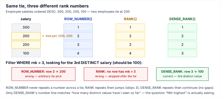
Mechanism first: the three ranking functions only disagree when there is a tie, and they disagree in three different ways — ROW_NUMBER() pretends the tie never happened and hands out a unique integer to each row in whatever order the tiebreak falls; RANK() gives tied rows the same number but then skips ahead by the tie's size; DENSE_RANK() gives tied rows the same number and does not skip. Only DENSE_RANK()'s output answers the question "how many distinct values have I seen so far?" — which is exactly what "the Nth-highest salary" is asking.
Traced worked example
Employee salaries, ordered descending: 300, 200, 200, 100 — two employees tie at 200. Asking for the 3rd-highest distinct salary (the correct answer is 100):
| salary | ROW_NUMBER() | RANK() | DENSE_RANK() |
|---|---|---|---|
| 300 | 1 | 1 | 1 |
| 200 | 2 | 2 | 2 |
| 200 | 3 | 2 | 2 |
| 100 | 4 | 4 | 3 |
Filter each result set for row/rank = 3: ROW_NUMBER returns the second 200 row — wrong, that value already had rank 2. RANK has no row numbered 3 at all — it jumped straight from 2 to 4 — so the query returns nothing. Only DENSE_RANK lands on 100, the actual 3rd distinct value.
-- General template: Nth-highest DISTINCT value via DENSE_RANK
SELECT salary
FROM (
    SELECT salary,
           DENSE_RANK() OVER (ORDER BY salary DESC) AS rnk
    FROM Employee
) ranked
WHERE rnk = 2;   -- swap 2 for N; wrap in SELECT (...) AS x to get NULL instead of no rows when N is out of range
Use ROW_NUMBER() only when you deliberately want "exactly one row, tie or not" (e.g. picking any one representative row per group). Use RANK() when the output should expose competition-style gaps (Olympic scoring: two golds means the next medal is bronze, not silver). Use DENSE_RANK() whenever the question is phrased around distinct values — "2nd highest salary," "3rd most recent distinct order date," "top-3 distinct price tiers."
2. Filter placement: WHERE vs ON in outer joins
Mechanism first: conceptually, an outer join's ON clause runs during the join — it decides which rows on the optional side get attached, but every row on the preserved (left) side survives regardless, with NULLs filled in where nothing matched. WHERE runs after the join is already complete, over the joined result — including those NULL-filled rows. A predicate on the optional table's column, written in WHERE, is evaluated against those NULLs too. In SQL's three-valued logic, NULL = anything is UNKNOWN, and WHERE discards any row that isn't TRUE — so it silently deletes exactly the unmatched-left rows an outer join exists to keep, collapsing the LEFT JOIN down to INNER JOIN behavior.
Traced worked example — Unused Accounts
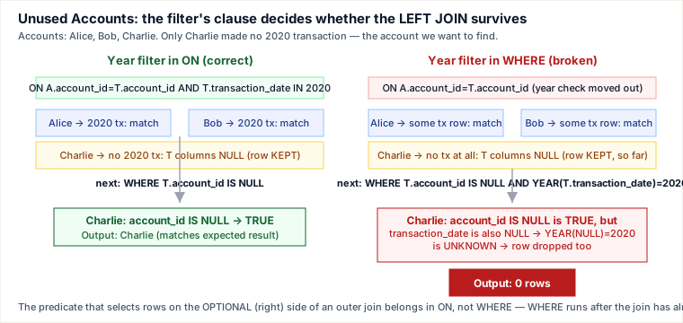
Find accounts with no transaction in 2020. Accounts: Alice, Bob, Charlie; only Charlie made no 2020 transaction. Written correctly, the year predicate sits in ON:
SELECT a.account_name
FROM Accounts a
LEFT JOIN Transactions t
       ON a.account_id = t.account_id
      AND t.transaction_date >= '2020-01-01'
      AND t.transaction_date <  '2021-01-01'
WHERE t.account_id IS NULL
ORDER BY a.account_name;
(The half-open range here is also the sargable rewrite of YEAR(transaction_date) = 2020 — wrapping the column in YEAR() defeats a B-tree index on transaction_date because the index is ordered by the raw value, not the function's output; see the Query Execution deep dive's sargability section.)
Now watch what happens if the year condition is written in WHERE instead, alongside the IS NULL check that is supposed to find the unused accounts:
SELECT a.account_name
FROM Accounts a
LEFT JOIN Transactions t
       ON a.account_id = t.account_id
WHERE t.account_id IS NULL
  AND YEAR(t.transaction_date) = 2020;   -- moved from ON to WHERE
For Charlie, t.account_id IS NULL is TRUE — but because the whole t row is NULL, t.transaction_date is NULL too, so YEAR(NULL) = 2020 evaluates to UNKNOWN. TRUE AND UNKNOWN is UNKNOWN, which WHERE treats as "reject." Charlie's row — the only row that should have survived — is dropped, and the query returns zero rows every time, regardless of the data.
The rule generalizes past this one problem: any predicate that should only narrow the optional side's rows, without affecting which left-side rows survive, belongs in ON. A predicate that should apply to the join's final result (after deciding survivorship) belongs in WHERE. WHERE t.account_id IS NULL is safe in WHERE precisely because it is testing the outcome of the join (did anything match?), not filtering the optional table's own columns before that outcome is decided.
3. Self-join fan-out and DISTINCT
Mechanism first: a self-join matches every qualifying row on one side against every qualifying row on the other side that shares the join key. When a middle entity appears on both sides with more than one partner each, the join doesn't add those partners — it multiplies them, one combined row per (left-partner, right-partner) pair. That multiplication is fan-out, and it is invisible until you count.
Worked example — Second Degree Follower
A second-degree follower both follows someone and is followed by someone; report each such user with their follower count:
SELECT f1.follower AS follower,
       COUNT(DISTINCT f2.follower) AS num
FROM Follow f1
JOIN Follow f2 ON f1.follower = f2.followee
GROUP BY f1.follower
ORDER BY f1.follower;
Illustrative data for user Bob: Bob follows 2 people (Alice, Cena) — that's 2 rows of f1 with f1.follower = 'Bob'. Separately, 2 people follow Bob (Donald, Edward) — that's 2 rows of f2 with f2.followee = 'Bob'. The join condition f1.follower = f2.followee pairs every one of Bob's 2 "follows" rows against every one of Bob's 2 "followed-by" rows: 2 × 2 = 4 combined rows, all carrying f1.follower = 'Bob'. COUNT(f2.follower) over those 4 rows would report 4 — but Bob only has 2 distinct followers (Donald and Edward each get counted twice, once per person Bob follows). Only COUNT(DISTINCT f2.follower) collapses the duplicates back to the true count, 2.
When a half-open condition replaces DISTINCT
DISTINCT is the right tool when the fan-out creates duplicate values you must collapse (as above). A different self-join shape — finding mutual pairs ("users who follow each other back") — fans out differently: it produces both (A, B) and (B, A) as separate, non-duplicate rows, so DISTINCT alone won't remove them (they aren't identical rows). The fix there is a half-open ordering condition on the join itself:
SELECT f1.follower AS user_a, f1.followee AS user_b
FROM Follow f1
JOIN Follow f2
  ON f1.follower = f2.followee
 AND f1.followee = f2.follower
WHERE f1.follower < f1.followee;   -- keeps (A,B), drops the mirror-image (B,A)
The distinction that matters: use DISTINCT when the join produces genuinely repeated values for the same logical answer (Second Degree Follower); use an ordering condition like a < b when the join produces two symmetric-but-distinct rows describing the same unordered pair.
4. Conditional aggregation cost and low-cardinality index selectivity
Mechanism first: SUM(CASE WHEN ... THEN 1 ELSE 0 END) (or the equivalent COUNT(CASE WHEN ... THEN 1 END)) cannot skip a single row — every row in the group must be inspected to decide which branch it falls into, so the cost is always O(rows in the group), one full pass, regardless of how skewed the categories are. That part is unavoidable and cheap: three SUM(CASE...) columns computed in the same query cost the same one pass as computing just one.
The senior-level question that follows is different: would an index help this query go faster? For Employee Attendance Record — pivoting status ('Present'/'Absent'/'Late') into per-status counts — a covering index on Attendance(employee_id, status) helps, but not by making the conditional aggregation itself skip rows; it helps by letting the LEFT JOIN probe per employee via an ordered index walk that also satisfies ORDER BY employee_id, avoiding a separate sort.
Contrast that with Green Product Identification, filtering Inventory on two 2-value enum columns, organic and biodegradable. A composite index (organic, biodegradable) has at most 4 distinct key combinations. If roughly a quarter of rows are (Y, Y), the optimizer's selectivity estimate for that predicate is around 25% of the table — nowhere near the roughly-single-digit-percent crossover below which an index scan beats a sequential scan (see the Query Execution deep dive's selectivity crossover). An index seek that then does random heap I/O for a quarter of all rows costs more than one linear pass over every page. The planner will — correctly — pick a sequential scan and ignore the index. A covering index can still help here, but for a different reason: if the index carries all needed columns (e.g. (organic, biodegradable, product_id)), the engine can answer straight from the index without touching the heap at all (an index-only scan) — it isn't narrowing the search, it's skipping the heap lookup entirely.
5. Portability and edge correctness
Two patterns look bulletproof on the sample data in the problem statement and quietly break somewhere realistic.
Latent bug 1 — row-value IN is not portable
Game Play Analysis IV (fraction of players who logged in again the day after their first login) is often solved with a row-constructor membership test:
SELECT ROUND(
         COUNT(DISTINCT a.player_id)
         / (SELECT COUNT(DISTINCT player_id) FROM Activity), 2) AS fraction
FROM Activity a
WHERE (a.player_id, DATE_SUB(a.event_date, INTERVAL 1 DAY)) IN (
        SELECT player_id, MIN(event_date)
        FROM Activity
        GROUP BY player_id
);
(a, b) IN (SELECT c, d ...) works on MySQL and PostgreSQL, but SQL Server has no multi-column IN — this is a straight syntax error there, not a silent wrong answer. The portable rewrite replaces the row-value membership test with a join to a first-login CTE:
WITH first_login AS (
    SELECT player_id, MIN(event_date) AS first_date
    FROM Activity
    GROUP BY player_id
)
SELECT ROUND(
         COUNT(DISTINCT a.player_id)
         / (SELECT COUNT(*) FROM first_login), 2) AS fraction
FROM Activity a
JOIN first_login f
  ON a.player_id = f.player_id
 AND a.event_date = DATE_ADD(f.first_date, INTERVAL 1 DAY);
Same result, no row-constructor syntax, and it runs unmodified on SQL Server.
Latent bug 2 — the consecutive-calendar-days assumption
High School Attendance (3+ consecutive absent days) is the classic gaps-and-islands trick: subtract a per-student ROW_NUMBER() from the actual attendance_date; rows in the same unbroken run share the same result, because each step forward in the run advances both the date and the row number by exactly one day.
WITH absents AS (
    SELECT student_id, attendance_date,
           ROW_NUMBER() OVER (PARTITION BY student_id ORDER BY attendance_date) AS rn
    FROM Attendance
    WHERE status = 'Absent'
)
SELECT student_id, MIN(attendance_date) AS start_date
FROM absents
GROUP BY student_id, DATE_SUB(attendance_date, INTERVAL rn DAY)
HAVING COUNT(*) >= 3;
This is only correct if the table has exactly one row per consecutive calendar day when a student is absent. If attendance is only ever recorded on school days — no rows exist for weekends or holidays — then Friday, Monday, Tuesday absences are three consecutive school days but not three consecutive calendar dates: subtracting rn from the raw date no longer produces a constant value across that run, and it silently splits into two islands, undercounting the streak. The robust fix ranks over the distinct school-day calendar, not the raw date, so the grouping key advances by exactly 1 per school day regardless of the calendar gap between them:
WITH school_days AS (
    SELECT DISTINCT attendance_date FROM Attendance
),
ranked_days AS (
    SELECT attendance_date,
           DENSE_RANK() OVER (ORDER BY attendance_date) AS day_rnk
    FROM school_days
),
absents AS (
    SELECT a.student_id, a.attendance_date, r.day_rnk,
           ROW_NUMBER() OVER (PARTITION BY a.student_id ORDER BY a.attendance_date) AS rn
    FROM Attendance a
    JOIN ranked_days r ON a.attendance_date = r.attendance_date
    WHERE a.status = 'Absent'
)
SELECT student_id, MIN(attendance_date) AS start_date
FROM absents
GROUP BY student_id, (day_rnk - rn)
HAVING COUNT(*) >= 3;
day_rnk - rn stays constant across a run of consecutive school days even when calendar dates jump over a weekend, because both counters advance in lockstep with the school-day calendar rather than with raw dates.
Pitfalls
- ROW_NUMBER for a "distinct Nth" question. It never repeats a number, so a tie silently picks one arbitrary row instead of collapsing correctly — the single most common wrong answer to "2nd highest salary."
- RANK for a "distinct Nth" question. It repeats then skips, so filtering for rank
= Ncan match zero rows even though N distinct values exist. - A right-table predicate in WHERE on an outer join. It silently turns the join into an
INNER JOIN; the fix is moving it intoON, not adding more conditions toWHERE. - Forgetting DISTINCT after a self-join. Any self-join where the middle entity has more than one partner on either side fans out; skipping
DISTINCT(or the appropriate dedup condition) silently inflates counts. - Assuming an index always helps a filtered aggregate. On a low-cardinality column, the planner's own cost math says otherwise — verify with
EXPLAIN, don't assume. - Row-value
INand calendar-day-only trick logic ported blindly to a new engine or dataset. Both look correct until the target engine (SQL Server) or the real data (non-calendar-daily records) breaks the assumption baked into the pattern.
Judgment layer: how a senior engineer decides
- Which ranking function: question is phrased around distinct values ("Nth highest," "top-N distinct tiers") →
DENSE_RANK(). Question wants competition-style medal gaps ("rank" in a leaderboard where ties should visibly cost the next competitor a spot) →RANK(). Question wants exactly one arbitrary representative row per partition, ties irrelevant →ROW_NUMBER()(e.g. "keep only the latest row per key"). - Would an index help this low-cardinality filter: estimate the number of distinct key combinations and the resulting selectivity. A handful of distinct keys covering a large fraction of rows each (2-value enums, booleans, status flags with a few common values) → a plain index rarely beats a sequential scan; a covering index can still pay off via an index-only scan if it removes heap lookups entirely. High-cardinality columns (IDs, timestamps, most string columns) → a plain index usually wins comfortably.
- DISTINCT vs a half-open join condition: the join produces repeated identical output rows for one logical answer →
DISTINCT/COUNT(DISTINCT ...). The join produces two distinct-but-symmetric rows for one unordered pair → aWHERE a < bstyle condition, which is both a correctness fix and half the row-count cost of computing then deduplicating.
Takeaways
DENSE_RANK()is the only one of the three ranking functions whose numbering matches "how many distinct values have I seen" — reach for it whenever the question says "distinct."- A predicate on the optional side of an outer join belongs in
ON; the same predicate inWHEREsilently reverts the join to inner-join behavior via three-valuedNULLlogic. - A self-join fans out whenever the shared key has multiple partners on both sides — know whether the fix is
DISTINCT(collapsing true duplicates) or a half-open ordering condition (removing symmetric mirror rows). - Conditional aggregation always costs one full pass; whether an index helps depends on selectivity, not on how clever the
CASEexpression is — low-cardinality columns usually don't benefit from a plain index.
Related pages
- SQL Practice Patterns I — NULL Traps, COUNT Semantics, Sargability & the Missing-Group Pattern (Deep Dive) — direct prerequisite companion this page continues
- SQL Practice Patterns III — Gaps-and-Islands (the Canonical Technique), DENSE_RANK n-th & Zero-Day Semantics (Deep Dive) — sibling deep dive on the gaps-and-islands technique used in pattern 5
- SQL Practice Patterns IV — Join Grain & Fan-out, GROUP_CONCAT Portability, NULL Ordering & Self-Join Cost (Deep Dive) — sibling deep dive on join fan-out, directly relevant to pattern 3
- Query Execution — Selectivity, the Cost Model, Join Algorithms, Spills & Sargability (Deep Dive) — the cost mechanics behind pattern 4's index-selectivity judgment
- Indexing & Storage — Fanout Arithmetic, Optimizer Stats, Composite/Skip Scans & NULL/OR Pitfalls (Deep Dive) — index selectivity mechanics behind pattern 4
Grounded in this guide's SQL Practice Problems slice — 2nd Highest Salary, Unused Accounts, Second Degree Follower, Green Product Identification, Employee Attendance Record, Game Play Analysis IV, and High School Attendance. Re-authored/Deepened for this guide.
🤖 Don't fully get this? Learn it with Claude
Stuck on SQL Practice Patterns II — Window-Function Ties, WHERE-vs-ON Placement, Self-Join Fan-out & Portability (Deep Dive)? Open Claude, copy a block below, and it'll teach you this exact concept — visually and interactively.
Build the mental picture, not memorization.
I just read a lesson on **SQL Practice Patterns II — Window-Function Ties, WHERE-vs-ON Placement, Self-Join Fan-out & Portability (Deep Dive)** (Databases) and want to truly understand it. Explain SQL Practice Patterns II — Window-Function Ties, WHERE-vs-ON Placement, Self-Join Fan-out & Portability (Deep Dive) from first principles using ONE vivid real-world analogy and a visual mental model — draw it as ASCII art or a clear step-by-step diagram — with a concrete example using real numbers. Then ask me one question to check I got the mental picture, and wait for my reply. If you're unsure or a claim isn't standard, say so and reason from first principles instead of guessing.
Socratic — adapts to where you're stuck.
Teach me **SQL Practice Patterns II — Window-Function Ties, WHERE-vs-ON Placement, Self-Join Fan-out & Portability (Deep Dive)** interactively. Ask me ONE guiding question at a time, wait for my answer, and adapt to my confusion — build the idea with me step by step instead of explaining it all at once. If you're unsure or a claim isn't standard, say so and reason from first principles instead of guessing.
Active recall exposes what you missed.
Quiz me on **SQL Practice Patterns II — Window-Function Ties, WHERE-vs-ON Placement, Self-Join Fan-out & Portability (Deep Dive)** with 5 questions, easy to tricky, ONE at a time. Tell me if each answer is right; at the end, explain clearly what I got wrong and why. If you're unsure or a claim isn't standard, say so and reason from first principles instead of guessing.
Intuition + hook + flashcards for long-term memory.
Help me remember **SQL Practice Patterns II — Window-Function Ties, WHERE-vs-ON Placement, Self-Join Fan-out & Portability (Deep Dive)** for the long term: give the one-sentence intuition, a memorable hook/mnemonic, a tiny worked example, and 3 active-recall flashcards (Q -> A). If you're unsure or a claim isn't standard, say so and reason from first principles instead of guessing.