Home › DSA › Foundations

An Overview of Big-O

Big-O notation is a mathematical notation that is used to describe the performance or complexity of an algorithm, specifically how long an algorithm takes to run as the input size grows. Understanding Big-O notation is essential for software engineers, as it allows them to analyze and compare the efficiency of different algorithms and make informed decisions about which one to use in a given situation. In this guide, we will cover the basics of Big-O notation and how to use it to analyze the performance of algorithms.

What is Big-O?

Big-O notation is a way of expressing the time (or space) complexity of an algorithm. It provides a rough estimate of how long an algorithm takes to run (or how much memory it uses), based on the size of the input. For example, an algorithm with a time complexity of means that the running time increases linearly with the size of the input.

What is time complexity?

Time complexity is a measure of how long an algorithm takes to run, based on the size of the input. It is expressed using Big-O notation, which provides a rough estimate of the running time. An algorithm with a lower time complexity will generally be faster than an algorithm with a higher time complexity.

What is space complexity?

Space complexity is a measure of how much memory an algorithm requires, based on the size of the input. Like time complexity, it is expressed using Big-O notation. An algorithm with a lower space complexity will generally require less memory than an algorithm with a higher space complexity.

Examples of time complexity

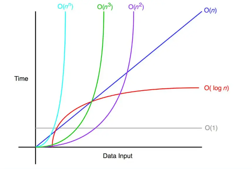
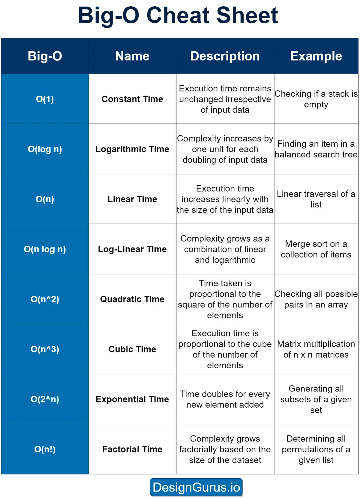
Here are some examples of how different time complexities are expressed using Big-O notation:

: Constant time. The running time is independent of the size of the input.
: Linear time. The running time increases linearly with the size of the input.
: Quadratic time. The running time is proportional to the square of the size of the input.
: Logarithmic time. The running time increases logarithmically with the size of the input.
: Exponential time. The running time increases exponentially in the size of the input.

Big-O notation uses mathematical notation to describe the upper bound of an algorithm’s running time. It provides a way to compare the running time of different algorithms, regardless of the specific hardware or implementation being used.

It’s important to note that Big-O notation only provides an upper bound on the running time of an algorithm. This means that an algorithm with a time complexity of could potentially run faster than an algorithm with a time complexity of in some cases, depending on the specific implementation and hardware being used.

Additionally, Big-O notation only considers the dominant term in the running time equation. For example, an algorithm with a running time of would be simplified to .

Example algorithms and their time complexities

1. Linear search -

Here are a few examples of algorithms along with their time complexities expressed using Big-O notation:

java

public class Solution {

  public static int linearSearch(int[] arr, int x) {
    for (int i = 0; i < arr.length; i++) {
      if (arr[i] == x) {
        return i;
      }
    }
    return -1;
  }

  public static void main(String[] args) {
    int[] arr = { 3, 5, 7, 9, 11 };
    int x = 7;
    System.out.println(linearSearch(arr, x));
  }
}

This linear search algorithm has a time complexity of , since the running time is directly proportional to the size of the input. If the input size is , the linear search will take n steps to complete.

2. Binary search -

java

public class Solution {

  public static int binarySearch(int[] arr, int x) {
    int low = 0;
    int high = arr.length - 1;
    while (low <= high) {
      int mid = (low + high) / 2;
      if (arr[mid] < x) {
        low = mid + 1;
      } else if (arr[mid] > x) {
        high = mid - 1;
      } else {
        return mid;
      }
    }
    return -1;
  }

  public static void main(String[] args) {
    int[] arr = { 2, 3, 4, 10, 40 };
    int x = 10;
    System.out.println(binarySearch(arr, x));
  }
}

This binary search algorithm has a time complexity of , since the running time increases logarithmically with the size of the input. If the input size is , it will take approximately steps to complete the binary search.

3. Bubble sort -

java

public class Solution {

  public static void bubbleSort(int[] arr) {
    int n = arr.length;
    for (int i = 0; i < n; i++) {
      for (int j = 0; j < n - i - 1; j++) {
        if (arr[j] > arr[j + 1]) {
          int temp = arr[j];
          arr[j] = arr[j + 1];
          arr[j + 1] = temp;
        }
      }
    }
  }

  public static void main(String[] args) {
    int[] arr = { 64, 34, 25, 12, 22, 11, 90 };
    bubbleSort(arr);
    for (int i : arr) {
      System.out.print(i + " ");
    }
  }
}

This bubble sort algorithm has a time complexity of $²$ , since the running time is quadratic in the size of the input. If the input size is n, it will take approximately n² steps to complete the bubble sort.

4. Quick Sort - on average, worst case

java

import java.util.ArrayList;
import java.util.List;

public class Solution {

  public static List<Integer> quickSort(List<Integer> arr) {
    if (arr.size() <= 1) {
      return arr;
    }
    int pivot = arr.get(arr.size() / 2);
    List<Integer> left = new ArrayList<>();
    List<Integer> middle = new ArrayList<>();
    List<Integer> right = new ArrayList<>();
    for (int x : arr) {
      if (x < pivot) left.add(x);
      else if (x > pivot) right.add(x);
      else middle.add(x);
    }
    List<Integer> sorted = new ArrayList<>();
    sorted.addAll(quickSort(left));
    sorted.addAll(middle);
    sorted.addAll(quickSort(right));
    return sorted;
  }

  public static void main(String[] args) {
    List<Integer> arr = List.of(3, 6, 8, 10, 1, 2, 1);
    List<Integer> sortedArr = quickSort(arr);
    System.out.println("Sorted array: " + sortedArr);
  }
}

This implementation of quick sort has a time complexity of , on average. In the worst case, the time complexity is , if the pivot is always the smallest or largest element in the array.

The quick sort algorithm works by selecting a pivot element and partitioning the array into three subarrays: one containing elements less than the pivot, one containing elements equal to the pivot, and one containing elements greater than the pivot. It then recursively sorts the left and right subarrays.

The time complexity of quick sort is determined by the number of recursive calls that are made. Each recursive call processes approximately elements, so the total number of recursive calls is approximately . The running time of each recursive call is , so the total running time is .

5. Fibonacci sequence -

Here is an implementation of an algorithm for calculating the n'th element of the Fibonacci sequence:

java

public class Solution {

  public static int fibonacci(int n) {
    if (n == 0) {
      return 0;
    } else if (n == 1) {
      return 1;
    } else {
      return fibonacci(n - 1) + fibonacci(n - 2);
    }
  }

  public static void main(String[] args) {
    int n = 10; // Example input
    System.out.println(
      "Fibonacci number at position " + n + " is " + fibonacci(n)
    );
  }
}

This implementation of the Fibonacci sequence has a time complexity of , which is exponential in the size of the input. This is because each call to fibonacci(n) results in two additional recursive calls to fibonacci(n-1) and fibonacci(n-2).

The time complexity of this algorithm is determined by the number of recursive calls that are made. Each recursive call processes one element, so the total number of recursive calls is approximately . The running time of each recursive call is , so the total running time is .

Example algorithms and their space complexities

Here are a few examples of algorithms along with their space complexities expressed using Big-O notation:

1. Linear search -

java

public class Solution {

  public static int linearSearch(int[] arr, int x) {
    for (int i = 0; i < arr.length; i++) {
      if (arr[i] == x) {
        return i;
      }
    }
    return -1;
  }

  public static void main(String[] args) {
    int[] arr = { 3, 4, 2, 7, 9 };
    int x = 7;
    int result = linearSearch(arr, x);
    System.out.println(
      result != -1 ? "Element found at index " + result : "Element not found"
    );
  }
}

This linear search algorithm has a space complexity of O(1), since it only requires a constant amount of memory regardless of the size of the input. It creates a single variable (i) to store the loop index, but the memory required for this variable is constant.

2. Fibonacci sequence -

This algorithm for calculating the nth element of the Fibonacci sequence has a space complexity of , since it uses recursion and the call stack grows with the size of the input. Each recursive call requires additional memory to store the state of the function, and the total amount of memory required increases linearly with the size of the input.

3. Merge sort -

java

public class Solution {

  public static void mergeSort(int[] arr) {
    if (arr.length > 1) {
      int mid = arr.length / 2;
      int[] left = new int[mid];
      int[] right = new int[arr.length - mid];

      System.arraycopy(arr, 0, left, 0, mid);
      System.arraycopy(arr, mid, right, 0, arr.length - mid);

      mergeSort(left);
      mergeSort(right);

      int i = 0,
        j = 0,
        k = 0;

      while (i < left.length && j < right.length) {
        if (left[i] < right[j]) {
          arr[k++] = left[i++];
        } else {
          arr[k++] = right[j++];
        }
      }

      while (i < left.length) {
        arr[k++] = left[i++];
      }

      while (j < right.length) {
        arr[k++] = right[j++];
      }
    }
  }

  public static void main(String[] args) {
    int[] arr = { 12, 11, 13, 5, 6, 7 };
    mergeSort(arr);
    for (int value : arr) {
      System.out.print(value + " ");
    }
  }
}

This merge sort algorithm has a space complexity of , since it creates two additional arrays (left and right) to store the left and right halves of the input during each recursive call. The memory required to store these arrays increases linearly with the size of the input.

4. Quick Sort - or

Quick sort has a space complexity of , on average. In the worst case, the space complexity is , if the pivot is always the smallest or largest element in the array. This is because the call stack grows with the number of recursive calls, and the number of recursive calls is logarithmic in the size of the input.

5. Create Matrix - $²$

java

public class Solution {

  public static int[][] createMatrix(int n) {
    int[][] matrix = new int[n][n];
    for (int i = 0; i < n; i++) {
      for (int j = 0; j < n; j++) {
        matrix[i][j] = 0;
      }
    }
    return matrix;
  }

  public static void main(String[] args) {
    int n = 3; // Example size
    int[][] matrix = createMatrix(n);
    for (int[] row : matrix) {
      for (int val : row) {
        System.out.print(val + " ");
      }
      System.out.println();
    }
  }
}

This algorithm creates an matrix filled with zeros. It does this by creating a new list of n zeros for each row of the matrix, and appending each row to the matrix.

The space complexity of this algorithm is , since the size of the matrix grows with the square of the size of the input (). The memory required to store the matrix increases proportionally to the size of the input.

Now, let's start with our first data structure, Array!

🤖 Don't fully get this? Learn it with Claude

Stuck on An Overview of Big-O? Open Claude, copy a block below, and it'll teach you this exact concept — visually and interactively.

🎨 Explain it visually

Build the mental picture, not memorization.

I just read a lesson on **An Overview of Big-O** (DSA) and want to truly understand it. Explain An Overview of Big-O from first principles using ONE vivid real-world analogy and a visual mental model — draw it as ASCII art or a clear step-by-step diagram — with a concrete example using real numbers. Then ask me one question to check I got the mental picture, and wait for my reply. If you're unsure or a claim isn't standard, say so and reason from first principles instead of guessing.

🤔 Walk me through it (interactive)

Socratic — adapts to where you're stuck.

Teach me **An Overview of Big-O** interactively. Ask me ONE guiding question at a time, wait for my answer, and adapt to my confusion — build the idea with me step by step instead of explaining it all at once. If you're unsure or a claim isn't standard, say so and reason from first principles instead of guessing.

🧪 Quiz me & fix my gaps

Active recall exposes what you missed.

Quiz me on **An Overview of Big-O** with 5 questions, easy to tricky, ONE at a time. Tell me if each answer is right; at the end, explain clearly what I got wrong and why. If you're unsure or a claim isn't standard, say so and reason from first principles instead of guessing.

🧠 Make it stick

Intuition + hook + flashcards for long-term memory.

Help me remember **An Overview of Big-O** for the long term: give the one-sentence intuition, a memorable hook/mnemonic, a tiny worked example, and 3 active-recall flashcards (Q -> A). If you're unsure or a claim isn't standard, say so and reason from first principles instead of guessing.

📝 My notes

← Types of Data Structures Introduction to Algorithm Analysis →

An Overview of Big-O

What is Big-O?

What is time complexity?

What is space complexity?

Examples of time complexity

Example algorithms and their time complexities

1. Linear search -

2. Binary search -

3. Bubble sort -

4. Quick Sort - on average, worst case

5. Fibonacci sequence -

Example algorithms and their space complexities

1. Linear search -

2. Fibonacci sequence -

3. Merge sort -

4. Quick Sort - or

5. Create Matrix - ²

📝 My notes

5. Create Matrix - $²$